Ry/Bericht

Diese Zusammenstellung basiert auf Befunden einer laufenden Plagiatsanalyse (Stand: 2016-04-11) – es handelt sich insofern nicht um einen abschließenden Bericht. Zur weiteren Meinungsbildung wird daher empfohlen, den jeweiligen Stand der Analyse auf der Seite http://de.vroniplag.wikia.com/wiki/Ry zum Vergleich heranzuziehen.

Eine kritische Auseinandersetzung mit der Dissertation von Raycho Yonchev: Permeation of Organometallic Compounds through Phospholipid Membranes

Dissertation zur Erlangung des Grades eines Doktors der Naturwissenschaften des Fachbereichs Chemie der Universität-GH Essen (jetzt Universität Duisburg-Essen. Betreuer: Prof. Dr. Heinz Rehage, Referent: Prof. Dr. Heinz Rehage, Koreferent: Prof. Dr. Alfred V. Hirner. Tag der mündlichen Prüfung: 19.10.2005. Publikation: Essen 2005. → Download Deutsche Nationalbibliothek, → Download Universität Duisburg-Essen

4. Juli 2016: Doktorgrad aberkannt → "'Der Fakultätsrat hat einstimmig beschlossen, Herrn Yonchev aufgrund seines schweren wissenschaftlichen Fehlverhaltens den Doktortitel abzuerkennen." (Protokoll der 10. o. Sitzung des Fakultätsrates Chemie vom 19. Juli 2016, PDF)

DNB-Anmerkung: "Ursprünglich als Dissertation veröffentlicht, Doktorgrad wurde am 02.07.2018 entzogen."

Der Barcode drückt den Anteil der Seiten aus, die Fremdtextübernahmen enthalten, nicht den Fremdtextanteil am Fließtext. Je nach Menge des übernommenen Textes werden drei Farben verwendet:

• schwarz: bis zu 50 % Fremdtextanteil auf der Seite
• dunkelrot: zwischen 50 % und 75 % Fremdtextanteil auf der Seite
• hellrot: über 75 % Fremdtextanteil auf der Seite

Weiße Seiten wurden entweder noch nicht untersucht oder es wurde nichts gefunden. Blaue Seiten umfassen Titelblatt, Inhaltsverzeichnis, Literaturverzeichnis, Vakatseiten und evtl. Anhänge, die in die Berechnung nicht einbezogen werden.

Der Barcode stellt den momentanen Bearbeitungsstand dar. Er gibt nicht das endgültige Ergebnis der Untersuchung wieder, da Untersuchungen im VroniPlag Wiki stets für jeden zur Bearbeitung offen bleiben, und somit kein Endergebnis existiert.

79 Seiten mit Plagiatstext

Seiten mit weniger als 50% Plagiatstext

4 Seiten: 079 069 068 085

Seiten mit 50%-75% Plagiatstext

2 Seiten: 067 038

Seiten mit mehr als 75% Plagiatstext

73 Seiten: 087 011 019 088 053 066 065 063 062 061 003 027 043 057 064 058 029 054 022 060 080 070 076 071 052 005 006 059 008 030 026 007 020 004 021 051 050 032 024 023 025 031 049 048 047 046 028 039 018 017 055 056 084 083 037 016 015 035 044 041 040 042 045 034 036 014 013 012 010 009 072 073 033

Befunde

• Die Dissertation enthält zahlreiche wörtliche und sinngemäße Textübernahmen, die nicht als solche kenntlich gemacht sind. Als betroffen festgestellt wurden bisher (Stand: 11. April 2016) folgende Kapitel, die sich teilweise als vollständig oder nahezu vollständig übernommen erwiesen haben – siehe Klammervermerke:

• I. Introduction and motivation of the thesis

• I.1. Biomembranes

• I.1.1 Structure and composition (S. 3-9): Seiten 3, 4, 5, 6, 7, 8, 9 – [vollständig (S. 4-9 wörtlich)]
• I.1.2 Membrane models (S. 9-11): Seiten 9, 10, 11 – [vollständig (wörtlich)]
• I.1.3 Model membranes (S. 11-13): Seiten 11, 12, 13 – [vollständig (wörtlich)]

• I.2. Phospholipid properties relevant to biomembranes [Anf.] (S. 13): Seite 13 – [vollständig (wörtlich)]

• I.2.1 The hydrophobic effect (S. 14): Seite 14 – [vollständig (wörtlich)]
• I.2.2 Phase structures (S. 14-19): Seiten 14, 15, 16, 17, 18, 19 – [vollständig (wörtlich)]
• I.2.3 Phase transitions (S. 19-22): Seiten 19, 20, 21, 22 – [vollständig (wörtlich)]
• I.2.4 Motional properties and membrane fluidity (S. 22-26): Seiten 22, 23, 24, 25, 26 – [vollständig (wörtlich)]

• I.3. Biomembrane transport

• I.3.1 Transport pathways and mechanisms (S. 27): Seite 27 – [vollständig (wörtlich)]
• I.3.2 Passive transport (S. 27-30): Seiten 27, 28, 29, 30 – [vollständig (wörtlich)]
• I.3.3 Active transport (S. 30-31): Seiten 30, 31 – [vollständig]

• I.4. Aim of the thesis (S. 31-32): Seiten 31, 32 – [vollständig]

• II. Theoretical background [Anf.] (S. 33): Seite 33 – [nahezu vollständig (exkl. letzter Satz)]

• II.1. Molecular dynamics simulations (S. 34-36): Seiten 34, 35, 36 – [vollständig]
• II.2. Molecular dynamics studies of lipid bilayers

• II.2.1 Review (S. 36-39): Seiten 36, 37, 38, 39 – [vollständig]
• II.2.2 Force fields (S. 39-46): Seiten 39, 40, 41, 42, 43, 44, 45, 46 – [vollständig (S. 42-46 wörtlich)]
• II.2.3 System size and boundary conditions (S. 46-47): Seiten 46, 47 – [vollständig (wörtlich)]
• II.2.4 Macroscopic ensembles (S. 48-52): Seiten 48, 49, 50, 51, 52 – [nahezu vollständig (exkl. ein Satz) (wörtlich)]
• II.2.5 Simulation time steps (S. 52-53): Seiten 52, 53 – [vollständig (wörtlich)]
• II.2.6 Treatment of long-range interactions (S. 53-56): Seiten 53, 54, 55, 56 – [vollständig (wörtlich)]
• II.2.7 Limitations of the MD technique (S. 56-57): Seiten 56, 57 – [vollständig (wörtlich)]

• II.3. Permeation models [Anf.] (S. 57-58): Seiten 57, 58 – [vollständig (wörtlich)]

• II.3.1 Homogeneous solubility-diffusion model (S. 58-59): Seiten 58, 59 – [vollständig (wörtlich)]
• II.3.2 Inhomogeneous solubility-diffusion model (S. 59-61): Seiten 59, 60, 61 – [vollständig (wörtlich)]
• II.3.3 Defect model (S. 61-62): Seiten 61, 62 – [vollständig (wörtlich)]

• II.4. Simulation of permeation processes [Anf.] (S. 62): Seite 62 – [vollständig (wörtlich)]

• II.4.1 Equilibrium MD simulations (S. 62-63): Seiten 62, 63 – [vollständig (wörtlich)]
• II.4.2 Non-equilibrium MD simulations (S. 63-66): Seiten 63, 64, 65, 66 – [vollständig]

• III. MD simulations of permeation processes through phospholipid bilayer

• III.1. Simulation methods

• III.1.1 Membrane system (S. 67-68): Seiten 67, 68
• III.1.3 Equilibrium MD simulations (S. 69-70): Seiten 69, 70 – [vollständig]
• III.1.4 Non-equilibrium MD simulations (S. 71): Seite 71 – [vollständig (wörtlich)]

• III.2. Results

• III.2.1 Equilibrium MD simulations (S. 71-78): Seiten 71, 72, 73, 76
• III.2.2 Non-equilibrium MD simulations (S. 78-82): Seiten 79, 80

• III.3. Discussion (S. 83-85): Seiten 83, 84, 85 – [S. 83 und 84 vollständig]

• IV. General conclusions (S. 87): Seite 87 – [vollständig]

• V. Summary (S. 88-89): Seite 88.

Herausragende Quellen

• Die Düsseldorfer Dissertation Anézo (2003) ist lediglich im Literaturverzeichnis (Nr. 77) genannt und im Text an einer Stelle (S. 68) referenziert, dient aber als Quelle für fast 85 % aller Fragmente.

Herausragende Fundstellen

• Der Teil I ("Introduction and motivation of the thesis", S. 3-32) ist mit allen seinen Unterkapiteln vollständig (großteils wörtlich) übernommen, ebenso der Teil IV ("General conclusions", S. 87).

Statistik

• Es sind bislang 83 gesichtete Fragmente dokumentiert, die als Plagiat eingestuft wurden. Bei 82 von diesen handelt es sich um Übernahmen ohne Verweis auf die Quelle („Verschleierungen“ oder „Komplettplagiate“). Bei einem Fragment ist die Quelle zwar angegeben, die Übernahme jedoch nicht ausreichend gekennzeichnet („Bauernopfer“).

• Die untersuchte Arbeit hat 87 Seiten im Hauptteil. Auf 79 dieser Seiten wurden bislang Plagiate dokumentiert, was einem Anteil von 90,8% der Seiten entspricht.

• Die 87 Seiten lassen sich bezüglich des Anteils, der als Plagiat eingestuft ist, wie folgt einordnen:

100 % = 69 Seiten

97 % = 1 Seite (S. 51)

95 % = 1 Seite (S. 3)

86 % = 1 Seite (S. 33)

75 % = 1 Seite (S. 80)

73 % = 1 Seite (S. 38)

58 % = 1 Seite (S. 67)

38 % = 1 Seite (S. 69)

36 % = 1 Seite (S. 79)

21 % = 1 Seite (S. 85)

14 % = 1 Seite (S. 68)

0 % = 8 Seiten (S. 74, 75, 77, 78, 81, 82, 86, 89).

• Ausgehend von dieser Aufstellung lässt sich angeben, wieviel Text der untersuchten Arbeit gegenwärtig als plagiiert dokumentiert ist: es sind rund 87 % des Textes im Hauptteil der Arbeit.

• Die Dokumentation beinhaltet 3 Quellen.

Illustration

Folgende Grafik illustriert das Ausmaß und die Verteilung der dokumentierten Fundstellen. Die Farben bezeichnen den diagnostizierten Plagiatstyp:
(grau=Komplettplagiat, rot=Verschleierung, gelb=Bauernopfer)

Die Nichtlesbarkeit des Textes ist aus urheberrechtlichen Gründen beabsichtigt.

Zum Vergrößern auf die Grafik klicken.

Anmerkung: Die Grafik repräsentiert den Analysestand vom 11. April 2016.

Definition von Plagiatkategorien

Die hier verwendeten Plagiatkategorien basieren auf den Ausarbeitungen von Wohnsdorf / Weber-Wulff: Strategien der Plagiatsbekämpfung, 2006. Eine vollständige Beschreibung der Kategorien findet sich im VroniPlag-Wiki. Die Plagiatkategorien sind im Einzelnen:

Übersetzungsplagiat

Ein Übersetzungsplagiat entsteht durch wörtliche Übersetzung aus einem fremdsprachlichen Text. Natürlich lässt hier die Qualität der Übersetzung einen mehr oder weniger großen Interpretationsspielraum. Fremdsprachen lassen sich zudem höchst selten mit mathematischer Präzision übersetzen, so dass jede Übersetzung eine eigene Interpretation darstellt. Zur Abgrenzung zwischen Paraphrase und Kopie bei Übersetzungen gibt es ein Diskussionsforum.

Komplettplagiat

Text, der wörtlich aus einer Quelle ohne Quellenangabe übernommen wurde.

Verschleierung

Text, der erkennbar aus fremder Quelle stammt, jedoch umformuliert und weder als Paraphrase noch als Zitat gekennzeichnet wurde.

Bauernopfer

Text, dessen Quelle ausgewiesen ist, der jedoch ohne Kenntlichmachung einer wörtlichen oder sinngemäßen Übernahme kopiert wurde.

Quellen nach Fragmentart

Die folgende Tabelle schlüsselt alle gesichteten Fragmente zeilenweise nach Quellen und spaltenweise nach Plagiatskategorien auf.

• ÜP = Übersetzungsplagiat,
• KP = Komplettplagiat,
• VS = Verschleierung,
• BO = Bauernopfer,
• KW = Keine Wertung,
• KeinP = Kein Plagiat.

Tabelle: Ry: Quellen / Fragmente (dynamische Auszählung)

Quelle	Jahr	ÜP	KP	VS	BO	KW	KeinP	∑	ZuSichten	Unfertig
Accelrys Inc. - Forcefield-Based Simulations	1998	0	5	5	1	0	0	11	0	0
Anézo	2003	0	48	24	0	0	0	72	0	0
Biosym MSI - Integration Algo	1995	0	0	0	0	1	0	1	0	1
∑	-	0	53	29	1	1	0	84	0	1

Fragmentübersicht

83 gesichtete, geschützte Fragmente

Fragment	SeiteArbeit	ZeileArbeit	Quelle	SeiteQuelle	ZeileQuelle	Typus
Ry/Fragment 003 02	3	2-20	Anézo 2003	9 ff.	9: 12 ff.; 10: 20 ff.; 11: 1 ff.	Verschleierung
Ry/Fragment 004 01	4	1 ff. (entire page)	Anézo 2003	11 f.	11: 5 ff.; 12: 1 ff.; 13: 1 ff.	KomplettPlagiat
Ry/Fragment 005 01	5	1 ff. (entire page)	Anézo 2003	13	10ff	KomplettPlagiat
Ry/Fragment 006 01	6	1 ff. (entire page)	Anézo 2003	14	1ff	KomplettPlagiat
Ry/Fragment 007 01	7	1 ff. (entire page)	Anézo 2003	14 f., 18, 20	14: 11 ff.; 15: 1 ff.; 18: 7 ff.; 20: 5 ff.	KomplettPlagiat
Ry/Fragment 008 01	8	1 ff. (entire page)	Anézo 2003	20 f.	20: 8 ff.; 21: 1 ff.	KomplettPlagiat
Ry/Fragment 009 01	9	1 ff. (entire page)	Anézo 2003	21, 22, 24	21:19ff; 22:1ff, 24:22-27	KomplettPlagiat
Ry/Fragment 010 01	10	1 ff. (entire page)	Anézo 2003	24, 25	24:28-30; 25:1ff	KomplettPlagiat
Ry/Fragment 011 01	11	1 ff. (entire page)	Anézo 2003	25, 26	25:27-34, 26:1 ff	KomplettPlagiat
Ry/Fragment 012 01	12	1 ff. (entire page)	Anézo 2003	26, 27	26:11ff; 27:1ff;	KomplettPlagiat
Ry/Fragment 013 01	13	1 ff. (entire page)	Anézo 2003	27, 28	27:18f; 28:1ff	KomplettPlagiat
Ry/Fragment 014 01	14	1 ff. (entire page)	Anézo 2003	28, 29	28:14ff; 29:	KomplettPlagiat
Ry/Fragment 015 01	15	1 ff. (entire page)	Anézo 2003	29, 30	29:11ff; 30:1ff	KomplettPlagiat
Ry/Fragment 016 01	16	1 ff. (entire page)	Anézo 2003	30, 31	30:8ff; 31:1ff	KomplettPlagiat
Ry/Fragment 017 01	17	1 ff. (entire page)	Anézo 2003	31	1 ff.	KomplettPlagiat
Ry/Fragment 018 01	18	1 ff. (entire page)	Anézo 2003	31, 32	31: 25-30; 32: 1 ff	KomplettPlagiat
Ry/Fragment 019 01	19	1 ff. (entire page)	Anézo 2003	31, 33	31: last lines, 33: 1 ff.	KomplettPlagiat
Ry/Fragment 020 01	20	1 ff. (entire page)	Anézo 2003	33, 34	33: 23 ff., 34: 1 ff.	KomplettPlagiat
Ry/Fragment 021 01	21	1 ff. (entire page)	Anézo 2003	34 f.	34: 22 ff.; 35: 1 ff.	KomplettPlagiat
Ry/Fragment 022 01	22	1 ff. (entire page)	Anézo 2003	35 f.	35: 16 ff.; 36: 1 ff.	KomplettPlagiat
Ry/Fragment 023 01	23	1 ff. (entire page)	Anézo 2003	36 f.	36: 11. ff.; 37: 1 ff.	KomplettPlagiat
Ry/Fragment 024 01	24	1 ff. (entire page)	Anézo 2003	37 f.	37: 13 ff.; 38: 1 ff.	KomplettPlagiat
Ry/Fragment 025 01	25	1 ff. (entire page)	Anézo 2003	38 f.	38: 11 ff.; 39: 1 ff.	KomplettPlagiat
Ry/Fragment 026 01	26	1 ff. (entire page)	Anézo 2003	39 f.	39: 24 ff.; 40: 1 ff.	KomplettPlagiat
Ry/Fragment 027 01	27	1 ff. (entire page)	Anézo 2003	40 f.	40: 20 ff.; 41: 1 ff.	KomplettPlagiat
Ry/Fragment 028 01	28	1 ff. (entire page)	Anézo 2003	41, 42	41:21 ff, 42:1 ff	KomplettPlagiat
Ry/Fragment 029 01	29	1 ff. (entire page)	Anézo 2003	42, 43	42: 12 ff., 43: 1 ff.	KomplettPlagiat
Ry/Fragment 030 01	30	1 ff. (entire page)	Anézo 2003	43 f.	43: 11 ff.; 44: 1 ff.;	KomplettPlagiat
Ry/Fragment 031 01	31	1 ff. (entire page)	Anézo 2003	44 f., 51	44: 27 ff.; 45: 1 ff.; 51: 7 ff.	Verschleierung
Ry/Fragment 032 01	32	1 ff. (entire page)	Anézo 2003	51 f.	51: 19 ff.; 52: 1 ff.	Verschleierung
Ry/Fragment 033 02	33	2-20	Anézo 2003	54, 55	54: 16 ff.; 55: 1 ff.	Verschleierung
Ry/Fragment 034 01	34	1 ff. (entire page)	Accelrys Inc. - Forcefield-Based Simulations 1998	3, 4, 192	3:4ff; 4:1-3; 192:18-22	Verschleierung
Ry/Fragment 035 01	35	1 ff. (entire page)	Accelrys Inc. - Forcefield-Based Simulations 1998	192, 193, 195	192: 22ff; 193:1-3,8-15,20ff; 195:7-13	Verschleierung
Ry/Fragment 036 01	36	1-6	Accelrys Inc. - Forcefield-Based Simulations 1998	195	15ff	Verschleierung
Ry/Fragment 036 07	36	7-20	Anézo 2003	56, 60	56:21-23; 60:8-19	Verschleierung
Ry/Fragment 037 01	37	1 ff. (entire page)	Anézo 2003	60, 61	60:16ff; 61:1ff	KomplettPlagiat
Ry/Fragment 038 01	38	1-12	Anézo 2003	61	61	KomplettPlagiat
Ry/Fragment 038 21	38	21-30	Anézo 2003	61, 62, 201	61:29-32; 62:1-4; 201:8-11	Verschleierung
Ry/Fragment 039 01	39	1-22	Anézo 2003	62, 56, 57	62: 2 ff; 56:28-29; 57: 1-4	Verschleierung
Ry/Fragment 039 23	39	23-26	Accelrys Inc. - Forcefield-Based Simulations 1998	54	13-16	Verschleierung
Ry/Fragment 040 01	40	1 ff. (entire page)	Accelrys Inc. - Forcefield-Based Simulations 1998	54, 55, 36,	54:16ff; 55:1ff; 36: 21ff	BauernOpfer
Ry/Fragment 041 01	41	1 ff.	Accelrys Inc. - Forcefield-Based Simulations 1998	37, 38	37, 38	Verschleierung
Ry/Fragment 042 01	42	1 ff. (entire page)	Accelrys Inc. - Forcefield-Based Simulations 1998	37, 38, 39	37:9-12; 38:1ff; 39:1ff	KomplettPlagiat
Ry/Fragment 043 01	43	1 ff. (entire page)	Accelrys Inc. - Forcefield-Based Simulations 1998	39, 40	39: 23 ff., 40: 1 ff.	KomplettPlagiat
Ry/Fragment 044 01	44	1 ff. (entire page)	Accelrys Inc. - Forcefield-Based Simulations 1998	40, 41	40:18ff; 41	KomplettPlagiat
Ry/Fragment 045 01	45	1 ff. (entire page)	Accelrys Inc. - Forcefield-Based Simulations 1998	41, 42	41:16ff; 42:1ff	KomplettPlagiat
Ry/Fragment 046 01	46	1-6	Accelrys Inc. - Forcefield-Based Simulations 1998	42	13-21	KomplettPlagiat
Ry/Fragment 046 07	46	7-30	Anézo 2003	63	7 ff	KomplettPlagiat
Ry/Fragment 047 01	47	1 ff. (entire page)	Anézo 2003	63, 64	63, 64	KomplettPlagiat
Ry/Fragment 048 01	48	1 ff. (entire page)	Anézo 2003	64, 65	64, 65	KomplettPlagiat
Ry/Fragment 049 01	49	1 ff. (entire page)	Anézo 2003	65, 66	65: 20-32; 66:1ff	KomplettPlagiat
Ry/Fragment 050 01	50	1 ff. (entire page)	Anézo 2003	66, 67	66:15ff; 67	KomplettPlagiat
Ry/Fragment 051 01	51	1-2; 4 ff.	Anézo 2003	67, 68	67:10ff; 68:1ff	KomplettPlagiat
Ry/Fragment 052 01	52	1 ff. (entire page)	Anézo 2003	68, 69, 70	68:6-9; 69:30-32; 70:1ff	KomplettPlagiat
Ry/Fragment 053 01	53	1 ff. (entire page)	Anézo 2003	70, 71	70:20-32; 71: 1-14	KomplettPlagiat
Ry/Fragment 054 01	54	1 ff. (entire page)	Anézo 2003	71-72	71:16-33; 72: 1-13	KomplettPlagiat
Ry/Fragment 055 01	55	1 ff (entire page)	Anézo 2003	72	72: 13 ff.; 73: 1-7	KomplettPlagiat
Ry/Fragment 056 01	56	1 ff. (entire page)	Anézo 2003	73, 74, 75	73:7-9,13-20; 74:20-32; 75:1ff	KomplettPlagiat
Ry/Fragment 057 01	57	1 ff. (entire page)	Anézo 2003	75	75: 3-23, 139:2 ff.	KomplettPlagiat
Ry/Fragment 058 01	58	1 ff. (entire page)	Anézo 2003	139	6ff	KomplettPlagiat
Ry/Fragment 059 01	59	1 ff. (entire page)	Anézo 2003	140	3 ff.	KomplettPlagiat
Ry/Fragment 060 01	60	1 ff. (entire page)	Anézo 2003	140, 141	140: 29 ff.; 141 1 ff.	KomplettPlagiat
Ry/Fragment 061 01	61	1 ff. (entire page)	Anézo 2003	141, 142	141:20-27; 142:1ff	KomplettPlagiat
Ry/Fragment 062 01	62	1 ff. (entire page)	Anézo 2003	142, 143	142:17-32; 143:1ff	KomplettPlagiat
Ry/Fragment 063 01	63	1 ff. (entire page)	Anézo 2003	143, 144, 145	143:12-19; 144:13-15,20-32; 145:	KomplettPlagiat
Ry/Fragment 064 01	64	1 ff. (entire page)	Anézo 2003	145, 147	145:4ff; 147:1-9	Verschleierung
Ry/Fragment 065 01	65	1 ff. (entire page)	Anézo 2003	147, 148, 150	147:10-14; 148:1-6; 150:1-11	Verschleierung
Ry/Fragment 066 01	66	1 ff. (entire page)	Anézo 2003	150	12 ff.	KomplettPlagiat
Ry/Fragment 067 06	67	6-12	Anézo 2003	78	78:1ff	Verschleierung
Ry/Fragment 068 01	68	1-4	Anézo 2003	78	7-10	Verschleierung
Ry/Fragment 069 14	69	14-21	Anézo 2003	156	5-15	Verschleierung
Ry/Fragment 070 01	70	1 ff. (complete page)	Anézo 2003	156, 157	156: 13ff; 157:1-9	Verschleierung
Ry/Fragment 071 01	71	1 ff.	Anézo 2003	157, 158, 159	157:10ff; 158:1-4,21ff; 159:1-3	Verschleierung
Ry/Fragment 072 01	72	1-9	Anézo 2003	159	4 ff.	Verschleierung
Ry/Fragment 073 00	73	(entire page)	Anézo 2003	160	-	Verschleierung
Ry/Fragment 076 01	76	1 ff.	Anézo 2003	165	2-11, 21ff	Verschleierung
Ry/Fragment 079 08	79	8-11	Anézo 2003	171	5-10	Verschleierung
Ry/Fragment 080 01	80	1-5 (entire page except figure)	Anézo 2003	171	171:8-9, 11-15	Verschleierung
Ry/Fragment 083 01	83	1 ff. (entire page)	Anézo 2003	48, 49	48: 9-17,26-31; 49: 1-7,15-21	Verschleierung
Ry/Fragment 084 01	84	1 ff.	Anézo 2003	49, 182, 183	49:18-26; 182:2-10; 183:12-24	Verschleierung
Ry/Fragment 085 01	85	1-6	Anézo 2003	182, 183	182: 30 ff. - 183: 1, 22-24	Verschleierung
Ry/Fragment 087 01	87	1ff (entire page)	Anézo 2003	183, 184	183: last paragraph; 184: 1ff	Verschleierung
Ry/Fragment 088 01	88	1 ff.	Anézo 2003	185, 186	185:1-12,20-22; 186: 1-8	Verschleierung

Textfragmente

Anmerkung zur Farbhinterlegung

Die Farbhinterlegung dient ausschließlich der leichteren Orientierung des Lesers im Text. Das Vorliegen einer wörtlichen, abgewandelten oder sinngemäßen Übernahme erschließt sich durch den Text.

Hinweis zur Zeilenzählung

Bei der Angabe einer Fundstelle wird alles, was Text enthält (außer Kopfzeile mit Seitenzahl), als Zeile gezählt, auch Überschriften. In der Regel werden aber Abbildungen, Tabellen, etc. inklusive deren Titel nicht mitgezählt. Die Zeilen der Fußnoten werden allerdings beginnend mit 101 durchnummeriert, z. B. 101 für die erste Fußnote der Seite.

83 gesichtete, geschützte Fragmente

[1.] Ry/Fragment 003 02

Verschleierung

Untersuchte Arbeit: Seite: 3, Zeilen: 2-20

Quelle: Anézo 2003 Seite(n): 9 ff., Zeilen: 9: 12 ff.; 10: 20 ff.; 11: 1 ff.

I. Introduction and motivation of the thesis I.1. Biomembranes I.1.1 Structure and composition Each cell is enclosed by lipid membrane, which assures a barrier between intracellular and extracellular environments and controls interactions and substance exchange between the cell and its surroundings. This description is valid for both prokaryotic and eukaryotic cells. On the molecular level biological membranes are too complex – they are composed of specific mixtures of lipids and proteins, which account for their diverse functions. Despite their complex composition, all biomembranes exhibit a universal construction principle. They essentially consist of a two dimensional matrix made up of a lipid bilayers, interrupted and coated by proteins. The hydrocarbon chains of the lipids confer a hydrophobic character on the membrane interior, whereas the polar headgroups found in the internal region have hydrophilic properties. This structural pattern results directly from the hydrophobic effect, whereby the non-polar lipid chains and the hydrophobic side chains of amino acid residues tend to minimize contacts with the aqueous phase. The components of the matrix are held together largely by non-covalent forces. Thus, biomembranes are not rigid structures, but are rather deformable. The hydrophobic effect accounts for most of the interaction energy that stabilizes the bilayer organization. Hydrogen bonding and electrostatic interactions contribute significantly to the [consolidation of this assembly in the interfacial region, while dispersive forces between the lipid hydrocarbon chains stabilize the core of the membrane.]

1.1 Biomembranes 1.1.1 Organization, structure, and functions 1.1.1.1 Organization Each biological cell is enclosed by its outer plasma membrane which provides a barrier between intracellular and extracellular domains and controls interactions between the cell and its surroundings. This description applies both to the relatively small prokaryotic cells, which have no cell nucleus, and to the much larger eukaryotic cells, which do have such a nucleus. [page 10:] 1.1.1.2 Structure On the molecular level, biological membranes are quite complex: they are composed of specific mixtures of lipids and proteins, which account for their diverse functions. Despite their complex composition, all biomembranes exhibit a universal construction principle. They essentially consist of a two-dimensional matrix made up of a lipid bilayer, interrupted and coated by proteins. The hydrocarbon chains of the lipids confer a hydrophobic character on the membrane interior, whereas the polar headgroups found in the interfacial region have hydrophilic properties. This structural pattern results directly from the so-called hydrophobic effect (see Section 1.2.1, page 28, for more details), whereby the apolar lipid chains and the hydrophobic side-chains of amino acid residues in proteins tend to minimize contacts with the aqueous phase. Figure 1.1 provides a simplified but informative picture of membrane structure. [page 11:] The components of the bilayer matrix are held together largely by non-covalent forces. Thus, biomembranes are not rigid structures, but are rather deformable. The hydrophobic effect accounts for most of the interaction energy that stabilizes the bilayer organization. Hydrogen bonding and electrostatic interactions, however, contribute significantly to the consolidation of this assembly in the interfacial region, while dispersive forces between the lipid hydrocarbon chains stabilize the core of the membrane.

Anmerkungen The source is not mentioned.

[2.] Ry/Fragment 004 01

KomplettPlagiat

Untersuchte Arbeit: Seite: 4, Zeilen: 1 ff. (entire page)

Quelle: Anézo 2003 Seite(n): 11 f., Zeilen: 11: 5 ff.; 12: 1 ff.; 13: 1 ff.

[Hydrogen bonding and electrostatic interactions contribute significantly to the] consolidation of this assembly in the interfacial region, while dispersive forces between the lipid hydrocarbon chains stabilize the core of the membrane. Even though each membrane exhibits functions unique to that membrane, general functions common to all membranes, can be distinguished. The first basic function of biomembranes is to provide different spatial compartments in living organisms. Compartmentalization (the physical separation of one compartment from another) supplies morphological identity to the cell and its organelles. Biomembranes act as selective barriers for the exchange of molecules between the different compartments, and ultimately, protect the internal microenvironments from the variability and fluctuations of their surroundings. They sustain concentration gradients of chemical species from one side to the other and the cell makes use of the membrane to create, maintain or utilize the energy stored in these concentration gradients. The bilayer matrix provides a two dimensional network in which various functional molecules such as enzymes are specifically distributed and oriented. Lipids act not only as solvent but also as anchors, activators and conformational stabilizers for proteins, which carry out specific catalytic and translocation functions. Another important aspect is the transduction of molecular information across and along membranes. For instance, receptors located on the cell surface receive extracellular signals that are conveyed to the cell interior, which alters it [sic] behavior in response. The major components of membranes are lipids and proteins. Depending on the type of membrane, their relative amounts vary significantly, ranging from about 20% protein (dry weight) to 80% protein. The most striking feature of membrane lipids is their very large diversity. Considering the possible number of structural and conformational lipid isomers, a hundred of components is involved in eukaryotic cells. In spite of this diversity, only a few classes of lipids predominate in membranes of a given type of organisms. The glycerophospholipids are the predominant phospholipids found in biological membranes. They are derivatives of glycerol phosphate and contain an asymmetric carbon atom. Two glycerol hydroxyls are linked to hydrophobic hydrocarbon chains.

Hydrogen bonding and electrostatic interactions, however, contribute significantly to the consolidation of this assembly in the interfacial region, while dispersive forces between the lipid hydrocarbon chains stabilize the core of the membrane. Figure 1.1: Schematic representation of a typical biomembrane. 1.1.1.3 Functions Even though each membrane exhibits functions unique to that membrane, general functions, common to all membranes, can be distinguished. The first basic function of biomembranes is to provide different spatial compartments in living organisms. Compartmentalization, i.e. the physical separation of one compartment from another, supplies morphological identity to the cell and its organelles. Biomembranes act as selective barriers for the exchange of molecules between the different compartments, and ultimately, protect the internal microenvironments from the variability and fluctuations of their surroundings. They sustain concentration gradients of chemical species from one side to the other and the cell makes use of the membrane to create, maintain, or utilize the energy stored in these concentration gradients. [page 12:] The bilayer matrix provides a two-dimensional network in which various functional molecules such as enzymes are specifically distributed and oriented. Lipids act not only as solvent but also as anchors, activators, and conformational stabilizers for proteins which carry out specific catalytic and translocation functions. Another important aspect is the transduction of molecular information across and along membranes. For instance, receptors located on the cell surface receive extracellular signals that are conveyed to the cell interior which alters its behavior in response. [...] 1.1.2 Composition The major components of membranes are lipids and proteins. Depending on the type of membrane, their relative amounts vary significantly, ranging from about 20% protein (dry weight) in myelin to 80% protein in mitochondria. [page 13:] 1.1.2.1 Membrane lipids The most striking feature of membrane lipids is their very large diversity. Considering the possible number of structural and conformational lipid isomers, a hundred of components is involved in eukaryotic cells. In spite of this diversity, only a few classes of lipids predominate in membranes of a given type of organisms. In this section, the main classes of lipids are described with regard to their molecular characteristics. Glycerophospholipids The glycerophospholipids are the predominant phospholipids found in biological membranes. They are derivatives of glycerol phosphate and contain an asymmetric carbon atom. Two glycerol hydroxyls are linked to hydrophobic hydrocarbon chains.

Anmerkungen The source is not given.

[3.] Ry/Fragment 005 01

KomplettPlagiat

Untersuchte Arbeit: Seite: 5, Zeilen: 1 ff. (entire page)

Quelle: Anézo 2003 Seite(n): 13, Zeilen: 10ff

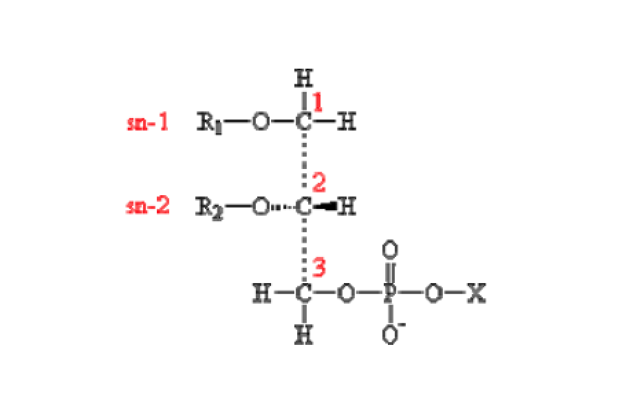
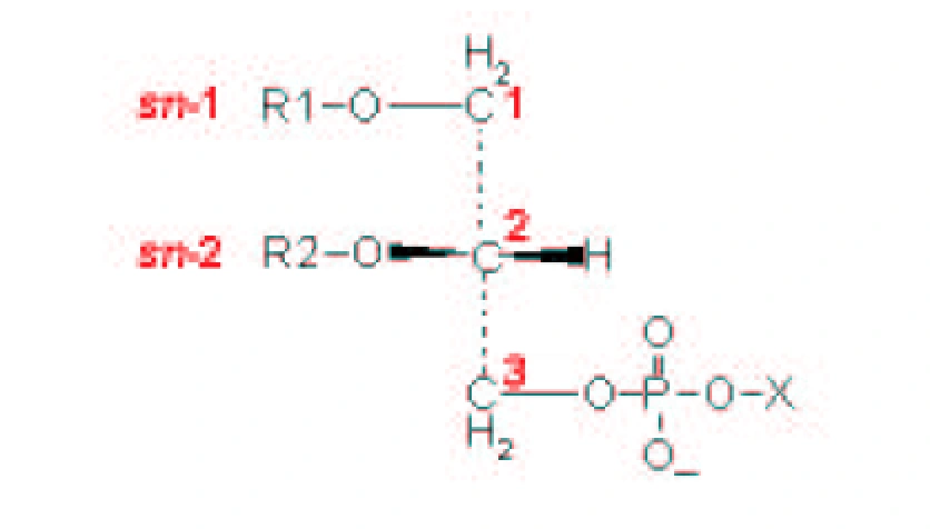
[A] stereospecific numbering (sn) of the glycerol carbon atoms is commonly used in the nomenclature of glycerophospholipids as indicated on Figure 1.1. In this nomenclature, the two hydrocarbon chains can be differentiated as sn-1 and sn-2 chains, the phosphate group being usually at the sn-3 position of the glycerol. In biological membranes, most of the glycerophospholipids are derivatives of sn-glycero-3-phosphatidic acid, the R-stereoisomer. The various glycerophospholipid types depend on the organic base, amino acid or alcohol (the X-group in Figure 1.2.) to which the phosphate is esterified and on the hydrocarbon chains which can be attached to the glycerol moiety through ester or ether linkages and vary widely in terms of length, branching or degree of unsaturation. Figure 1.1. General structure of glycerophospholipids with the glycerol backbone drawn in a Fisher [sic] projection. The stereospecific numbering (sn) of the glycerol carbon atoms, with the distinction between the sn-1 and sn-2 chains, is indicated.

A stereospecific numbering (sn) of the glycerol carbon atoms is commonly used in the nomenclature of glycerophospholipids, as indicated in Figure 1.2. In this nomenclature, the two hydrocarbon chains can be differentiated as sn-1 and sn-2 chains, the phosphate group being usually at the sn-3 position of the glycerol. In biological membranes, most of the glycerophospholipids are derivatives of sn-glycero-3-phosphatidic acid, the R-stereoisomer. The various glycerophospholipid types depend on the organic base, amino acid, or alcohol (the X-group in Figure 1.3) to which the phosphate is esterified and on the hydrocarbon chains which can be attached to the glycerol moiety through ester or ether linkages and vary widely in terms of length, branching, or degree of unsaturation. Figure 1.2: General structure of glycerophospholipids with the glycerol backbone drawn in a Fischer projection. The stereospecific numbering (sn) of the glycerol carbon atoms, with the distinction between the sn-1 and sn-2 chains, is indicated.

Anmerkungen No source is given.

[4.] Ry/Fragment 006 01

KomplettPlagiat

Untersuchte Arbeit: Seite: 6, Zeilen: 1 ff. (entire page)

Quelle: Anézo 2003 Seite(n): 14, Zeilen: 1ff

Figure 1.2. Generic structure of phospholipids. The phosphate can be esterified to the various X-groups listed to form the different classes of phospholipids. 1,2-Diacylglyceroophospholipids [sic] or phospholipids. These fatty acid esters of glycerol are the predominant lipids in most biomembranes. The phosphate is usually linked to one of the several groups listed in Figure 1.2, including choline, ethanolamine, the S-amino acid serine, and polyalcohols such as glycerol or inositol. The corresponding phospholipids are called phosphatidylcholines (commonly abbreviated PC), phosphatidylethanolamines (PE), phosphatidylserines (PS), phosphatidylglycerols (PG) and phosphatidylinositols (PI). PC and PE constitute the major components of biomembranes. The chemical structure of these polar headgroups determines what charge the phospholipid as a whole may carry. At physiological pH values, PC and PE carry a full negative charge on the phosphate and a full positive charge on the quaternary [ammonium – they are thus zwitterionic but electrically neutral. PS contain in addition to the negatively charged phosphate and the positively charged amino group, a negatively charged carboxyl group.]

Figure 1.3: Generic structure of phospholipids. The phosphate can be esterified to the various X-groups listed to form the different classes of phospholipids. 1,2-Diacylglycerophospholipids or phospholipids These fatty acid esters of glycerol are the predominant lipids in most biomembranes. The phosphate is usually linked to one of the several groups listed in Figure 1.3, including choline, ethanolamine, the S-amino acid serine, and polyalcohols such as glycerol or inositol. The corresponding phospholipids are called phosphatidylcholines (commonly abbreviated PC), phosphatidylethanolamines (PE), phosphatidylserines (PS), phosphatidylglycerols (PG), and phosphatidylinositols (PI). PC and PE constitute the major components of biological membranes. The chemical structure of these polar headgroups determines what charge the phospholipid as a whole may carry. At physiological pH values, PC and PE carry a full negative charge on the phosphate and a full positive charge on the quaternary ammonium: they are thus zwitterionic but electrically neutral. PS contain, in addition to the negatively charged phosphate and the positively charged amino group, a negatively charged carboxyl group.

Anmerkungen No source is given.

[5.] Ry/Fragment 007 01

KomplettPlagiat

Untersuchte Arbeit: Seite: 7, Zeilen: 1 ff. (entire page)

Quelle: Anézo 2003 Seite(n): 14 f., 18, 20, Zeilen: 14: 11 ff.; 15: 1 ff.; 18: 7 ff.; 20: 5 ff.

[At physiological pH values, PC and PE carry a full negative charge on the phosphate and a full positive charge on the quaternary] ammonium – they are thus zwitterionic but electrically neutral. PS contain in addition to the negatively charged phosphate and the positively charged amino group, a negatively charged carboxyl group. At neutral pH, PS exhibits an overall negative charge. PG and PI carry a net negative charge, since the alcoholic moiety does not carry any positive charge to counterbalance the negative charge on the phosphate. The headgroup charges are held at the interface between the aqueous and hydrophobic phases by the organization of the membrane bilayers. Phospholipids play therefore an important role in the determination of the surface charge of the membrane. The division of phospholipids into classes according to the structure of their headgroup represents only one level of complexity. On a second level, each phospholipid class exhibits various fatty acid chain compositions. The acyl chain lengths vary usually between 12 and 26 carbon atoms and may be saturated or unsaturated. The number of carbon-carbon double bonds can reach as many as 6 per chain. The most abundant saturated chains contain 16 or 18 carbon atoms and the major unsaturated species are C18:1, C18:2 and C20:4. In this notation the first figure refers to the chain length, while the second one indicates the number of double bonds. Nearly all naturally occurring double bonds are cis isomers disrupt the ordered packing of the lipid chains, perturbing the membrane structure. Some branched fatty acids such as isomyristate or isopalmitate may also occur in the lipid chain composition. Another variation is for instance the inclusion of a cyclopropane ring in the fatty acid chain. An overview of the lipid composition of mammalian plasma and intracellular organelle membranes, stemming from work of Jamieson and Robinson [1], shows that with a few exceptions, PC, PE and cholesterol appear to be the main components. PC are mainly composed of short chains and dipalmitoilphosphatidylcholine [sic] (DPPC), with saturated chains of 16 carbon atoms, is one of the principal component of this class of phospholipids. The principal unsaturated chains found in PC are 18:1 and 18:2. In PE, a relatively high proportion of polyunsaturated chains are found, especially 20:4 chains. The lipids found as membrane components are very diverse but have the same fundamental property in common – they are all amphipathic molecules, presenting separate polar and apolar regions and, for this reason, have natural propensity to form [bilayers structures in an aqueous environment.] 1. Jamieson, G. A.; Robinson, D. M. Mammalian Cell Membranes; Butterworth: London, 1977; Vol. 2.

At physiological pH values, PC and PE carry a full negative charge on the phosphate and a full positive charge on the quaternary ammonium: they are thus zwitterionic but electrically neutral. PS contain, in addition to the negatively charged phosphate and the positively charged amino group, a negatively charged carboxyl group. At neutral pH, PS exhibit an overall negative charge. PG and PI carry a net negative charge, since the alcoholic moiety does not carry any positive charge to counterbalance the negative charge on the phosphate. The headgroup charges are held at the interface between the aqueous and hydropho- [page 15:] bic phases by the organization of the membrane bilayer. Phospholipids play therefore an important role in the determination of the surface charge of the membrane. The division of phospholipids into classes according to the structure of their headgroup represents only one level of complexity. On a second level, each phospholipid class exhibits various fatty acid chain compositions. The acyl chain lengths vary usually between 12 and 26 carbon atoms and may be saturated or unsaturated. The number of carbon-carbon double bonds can reach as many as six per chain. The most abundant saturated chains contain 16 or 18 carbon atoms and the major unsaturated species are C18:1, C18:2, and C20:4. In this notation, the first figure refers to the chain length, while the second one indicates the number of double bonds. Nearly all naturally occurring double bonds are cis rather than trans. A cis double bond introduces a kink or bend in the molecule, so that cis isomers disrupt the ordered packing of the lipid chains, perturbing the membrane structure. Some branched fatty acids such as isomyristate or isopalmitate may also occur in the lipid chain composition. Another variation is for instance the inclusion of a cyclopropane ring in the fatty acid chain. [page 18:] Lipid composition of a few membranes An overview of the lipid composition of mammalian plasma and intracellular organelle membranes, stemming from the work of Jamieson and Robinson, is given in Table 1.1 [3]. Although these various membranes exhibit characteristic differences in their composition, some common features emerge. With a few exceptions, PC, PE, and cholesterol appear to be the main components. [...] PC are mainly composed of short chains and dipalmitoylphosphatidylcholine (DPPC), with saturated chains of 16 carbon atoms, is one of the principal component of this class of phospholipids. The principal unsaturated chains found in PC are 18:1 and 18:2. Sphingomyelin, in contrast, contains a great amount of long chains with 24 C-atoms with one double bond at the most. In PE, a relatively high proportion of polyunsaturated chains are found, especially 20:4 chains. [page 20:] Concluding remarks The lipids found as membrane components are very diverse but have the same fundamental property in common: they are all amphipathic molecules, presenting separate polar and apolar regions and, for this reason, have a natural propensity to form bilayer structures in an aqueous environment. [3] G. A. Jamieson and D. M. Robinson. Mammalian Cell Membranes, volume 2. Butterworth, London, 1977.

Anmerkungen The source is not given.

[6.] Ry/Fragment 008 01

KomplettPlagiat

Untersuchte Arbeit: Seite: 8, Zeilen: 1 ff. (entire page)

Quelle: Anézo 2003 Seite(n): 20 f., Zeilen: 20: 8 ff.; 21: 1 ff.

They can be differentiated by two main features – the size and electrical property of the headgroups, which may be charged, zwiterioninc [sic], or neutral, and the structure of the hydrocarbon chains which may have various lengths and different degrees of unsaturation. It should be emphasized that lipids having the same polar headgroup but different hydrocarbon chains, or vice versa, exhibit different physical and metabolic properties. The various membranes present in different organisms show characteristic patterns of lipid composition. To a first approximation, the specific functions exhibited by these membranes may arise from qualitative and quantitative differences an [sic] their composition. Many of these functions, however, might be appreciated in terms of the properties of the membrane in specific environments and not on the basis of the structure or the reactivity of its components per-se [sic] [2]. Membranes contain between 20 and 80 weight percent protein. Just as each membrane can be characterized by its lipid composition, each membrane can also be characterized by its protein contents. Thousands of different proteins are found as constituents of biological membranes. Whereas the primary role of membrane lipids is to provide the structural framework of the membrane in the form of stable bilayers, proteins provide the diversity of enzymes, transporters, receptors, and pores, i.e. the principal active components of the membrane. The covalent structure of the membrane proteins is similar to that of soluble proteins. Membrane proteins can be distinguished from non-membranous proteins by the nature of their association with the lipid bilayers. This association may be loose or tight. The proteins may be incorporated into the bilayers structure or simply associated to a lipid or protein component on the surface of the membrane. Membrane proteins are generally bound to the membrane through non-covalent forces, such as the hydrophobic force or electrostatic interactions. They may fold so as to present both a non-polar hydrophobic surface, which can interact with the apolar regions of the lipid bilayers, and polar or charged regions which can interact with the polar lipid headgroups at the interface of the membrane. There is also a certain number of membrane proteins which are covalently bound to the membrane via lipid anchors. Operationally, membrane proteins have been divided into two major classes – [peripheral (or extrinsic) proteins and integral (or intrinsic) proteins.] 2. Jain, M. K. Introduction to Biological Membranes, 2nd ed.; John Wiley & Sons: New York, 1988.

They can be differentiated by two main features: the size and electrical property of the headgroups which may be charged, zwitterionic, or neutral, and the structure of the hydrocarbon chains which may have various lengths and different degrees of unsaturation. It should be emphasized that lipids having the same polar headgroup but different hydrocarbon chains, or vice versa, exhibit different physical and metabolic properties. The various membranes present in different organisms show characteristic patterns of lipid composition. To a first approximation, the specific functions exhibited by these membranes may arise from qualitative and quantitative differences in their composition. Many of these functions, however, might be appreciated in terms of the properties of the membrane in specific environments and not on the basis of the structure or the reactivity of its components per se [4]. [page 21:] 1.1.2.2 Membrane proteins Membranes contain between 20 and 80 weight% protein. Just as each membrane can be characterized by its lipid composition, each membrane can be also characterized by its protein content. Thousands of different proteins are found as constituents of biological membranes. Whereas the primary role of membrane lipids is to provide the structural framework of the membrane in the form of a stable bilayer, proteins provide the diversity of enzymes, transporters, receptors, and pores, i.e. the principal active components of the membrane. The covalent structure of membrane proteins is similar to that of soluble proteins. Membrane proteins can be distinguished from non-membranous proteins by the nature of their association with the lipid bilayer. This association may be loose or tight. The proteins may be incorporated into the bilayer structure or simply associated to a lipid or protein component on the surface of the membrane. Membrane proteins are generally bound to the membrane through non-covalent forces, such as the hydrophobic force or electrostatic interactions. They may fold so as to present both a non-polar hydrophobic surface which can interact with the apolar regions of the lipid bilayer, and polar or charged regions which can interact with the polar lipid headgroups at the interface of the membrane. There is also a certain number of membrane proteins which are covalently bound to the membrane via lipid anchors. Operationally, membrane proteins have been divided into two major classes: peripheral (or extrinsic) proteins and integral (or intrinsic) proteins. [4] M. K. Jain. Introduction to Biological Membranes. John Wiley & Sons, New York, second edition, 1988.

Anmerkungen

[7.] Ry/Fragment 009 01

KomplettPlagiat

Untersuchte Arbeit: Seite: 9, Zeilen: 1 ff. (entire page)

Quelle: Anézo 2003 Seite(n): 21, 22, 24, Zeilen: 21:19ff; 22:1ff, 24:22-27

[Operationally, membrane proteins have been divided into two major classes –] peripheral (or extrinsic) proteins and integral (or intrinsic) proteins. This classification is based on the nature of their association with the lipid bilayers. The distinction between peripheral and integral proteins does not clearly define the mode of attachment to the bilayers, but rather the relative strength of the attachment, or the harshness of the treatment required to release the protein from membrane. Peripheral membrane proteins generally interact with the surface of the membrane only and are not integrated into the hydrophobic core of the lipid bilayers. They are thought to be weakly bound to the membrane surface by electrostatic interaction, either with the lipid headgroups or with other proteins. Such an association is rather loose and peripheral membrane proteins can be readily removed by washing the membrane, changing the ionic strength or the pH. Integral membrane proteins extend deeply into or completely through the lipid bilayers and are thus integrated into the bilayers structure. Generally they can be removed from the membrane only with detergents or stronger agents that disrupt the membrane structure. The portion of the protein integrated into the membrane is thus thermodynamically compatible with the hydrophobic core of the bilayers – one expects a preponderance of hydrophobic amino acid residues in the intramembranous portion of the protein. Integral membrane proteins can be further divided into two subclasses. Transmembrane proteins constitute one of these subclasses and, as their name implies, span the lipid bilayers of the membrane. The other subclass refers to anchored proteins. A portion of these proteins is embedded in the hydrophobic interior of the bilayers, without passing completely through the membrane. In most cases, the lipids provide a hydrophobic anchor by which the protein is attached to the membrane. I.1.2 Membrane models At the turn of the nineteenth century, Overton speculated on the lipid nature of biomembranes by observing a correlation between the rates at which various small molecules penetrate plant cells and their partition coefficients in an oil/water system [3]. 3. Overton, E. Vierteljahrsschr. Naturforsch. Ges. Zurich [sic] 1899, 44 , 88.

[page 21] Operationally, membrane proteins have been divided into two major classes: peripheral (or extrinsic) proteins and integral (or intrinsic) proteins. This classification is based on the nature of their association with the lipid bilayer. The distinction between peripheral and integral proteins does not clearly define the mode of attachment to the bilayer, but rather the relative strength of the attachment, or the harshness of the treatment required to release the protein from the membrane. Peripheral membrane proteins Peripheral membrane proteins generally interact with the surface of the membrane only and are not integrated into the hydrophobic core of the lipid bilayer. They are thought to be weakly bound to the membrane surface by electrostatic interactions, either with the lipid headgroups or with other proteins. Such an association is rather loose and peripheral membrane proteins can be readily removed by washing the membrane, changing the ionic strength or the pH. Integral membrane proteins Integral membrane proteins extend deeply into or completely through the lipid bilayer and are thus integrated into the bilayer structure. [page 22] Generally, they can be removed from the membrane only with detergents or stronger agents that disrupt the membrane structure. The portion of the protein integrated into the membrane is thus thermodynamically compatible with the hydrophobic core of the bilayer: one expects a preponderance of hydrophobic amino acid residues in the intramembranous portion of the protein. Integral membrane proteins can be further divided into two subclasses. Transmembrane proteins constitute one of these subclasses and, as their name implies, span the lipid bilayer of the membrane. The other subclass refers to anchored proteins. A portion of these proteins is embedded in the hydrophobic interior of the bilayer, without passing completely through the membrane. In most cases, the lipids provide a hydrophobic anchor by which the protein is attached to the membrane. [page 24] 1.1.5 Membrane models This section gives a brief historical overview of the main stages that have contributed to the actual conception of membrane model. At the turn of the nineteenth century, Overton speculated on the lipid nature of biomembranes by observing a correlation between the rates at which various small molecules penetrate plant cells and their partition coefficients in an oil/water system [13]. [13] E. Overton. Vierteljahrsschr. Naturforsch. Ges. Zürich, 44:88–135, 1899.

Anmerkungen No source is given.

[8.] Ry/Fragment 010 01

KomplettPlagiat

Untersuchte Arbeit: Seite: 10, Zeilen: 1 ff. (entire page)

Quelle: Anézo 2003 Seite(n): 24, 25, Zeilen: 24:28-30; 25:1ff

In 1925, Gorter and Grendel introduced for the first time the concept of lipid bilayers as structural basis of biomembranes [4]. They postulated that lipids in the human erythrocyte membrane are organized in the form of a bimolecular leaflet or lipid bilayers. In 1935, Davson and Danielli made a major contribution to the development of membrane models [5]. They found that a membrane such as the erythrocyte contains, besides lipids, a significant amount of proteins and included, therefore, proteins in their model. They suggested that proteins coat the surface of the lipid bilayers. This description was motivated by the new (at that time) knowledge of the β-sheet structure. In this model, the protein was thus not allowed to penetrate into the bilayers. In the 1960’s and 1970’s, new molecular insights into biological membranes were gained by the emergence of more sophisticated experimental techniques. Freeze-fracture electron microscopy revealed the existence of globular particles embedded within the lipid bilayers. Spectroscopic methods indicated that membrane proteins had an appreciable amount of α-helixes and that they were likely globular. The characterization of hydrophobic domains in membrane proteins also stimulated the integration of proteins into the membrane interior. At the same time, nuclear magnetic resonance measurements pointed out the fluid character of the lipid bilayers. In 1996 [sic], Green and co-workers attempted to integrate the protein structure into the membrane in a model built around lipid-protein complexes as the fundamental structural pattern [6]. Although this model did not give prominence to the lipid bilayers as the basic structure of the membrane, it did incorporate proteins inside the membrane structure, introducing the concept of integral membrane proteins. In 1970, Frye and Edidin performed a series of experiments on cell membrane fusion and suggested that membrane components can move laterally in the plane of the membrane [7]. In 1972, Singer and Nicolson amalgamated all these experimental observations and conceived a new model for the membrane structure, so called fluid mosaic model [8]. This model described the biological membrane as a two-dimensional fluid or liquid crystal in which lipids as well as protein components are constrained within the plane of the membrane, but are free to diffuse laterally. The notions of integral and peripheral [membrane proteins were asserted and it was also suggested that some proteins might pass completely through the membrane.] 4. Gorter, E.; Grendel, F. J. Exp. Med. 1925, 41, 439. 5. Danielli, J. F.; Davson, H. J. Cell. Comp. Physiol. 1935, 5, 495. 6. Green, D. E.; Perdue, J. Proc. Natl. Acad. Sci. USA 1996 [sic], 55, 1295. 7. Frye, L. D.; Edidin, M. J. Cell. Sci. 1970, 7, 319. 8. Singer, S. J.; Nicolson, G. L. Science 1972, 175 , 720.

[page 24] In 1925, Gorter and Grendel introduced for the first time the concept of lipid bilayer as structural basis of biomembranes [14]. They postulated that lipids in the human erythrocyte membrane are organized in the form of a bimolecular leaflet or lipid bilayer. [page 25] In 1935, Davson and Danielli made a major contribution to the development of membrane models [15]. They found that a membrane such as the erythrocyte contains, besides lipids, a significant amount of proteins and included, therefore, proteins in their model. They suggested that proteins coat the surface of the lipid bilayer. This description was motivated by the new (at that time) knowledge of the β-sheet structure. In this model, the protein was thus not allowed to penetrate into the lipid bilayer. In the 1960’s and 1970’s, new molecular insights into biological membranes were gained by the emergence of more sophisticated experimental techniques. Freeze-fracture electron microscopy revealed the existence of globular particles embedded within the lipid bilayer. Spectroscopic methods indicated that membrane proteins had an appreciable amount of α-helixes and that they were likely globular. The characterization of hydrophobic domains in membrane proteins also stimulated the integration of proteins into the membrane interior. At the same time, nuclear magnetic resonance measurements pointed out the fluid character of the lipid bilayer. In 1966, Green and co-workers attempted to integrate the protein structure into the membrane in a model built around lipid-protein complexes as the fundamental structural pattern [16]. Although this model did not give prominence to the lipid bilayer as the basic structure of the membrane, it did incorporate proteins inside the membrane structure, introducing the concept of integral membrane proteins. In 1970, Frye and Edidin performed a series of experiments on cell membrane fusion and suggested that membrane components can move laterally in the plane of the membrane [17]. In 1972, Singer and Nicolson amalgamated all these experimental observations and conceived a new model for the membrane structure, the so-called fluid mosaic model [18]. This model described the biological membrane as a two-dimensional fluid or liquid crystal in which lipid as well as protein components are constrained within the plane of the membrane, but are free to diffuse laterally. The notions of integral and peripheral membrane proteins were asserted and it was also suggested that some proteins may pass completely through the membrane. [14] E. Gorter and F. Grendel. J. Exp. Med., 41:439–443, 1925. [15] J. F. Danielli and H. Davson. J. Cell. Comp. Physiol., 5:495–508, 1935. [16] D. E. Green and J. Perdue. Proc. Natl. Acad. Sci. USA, 55:1295–1302, 1966. [17] L. D. Frye and M. Edidin. J. Cell. Sci., 7:319–335, 1970. [18] S. J. Singer and G. L. Nicolson. Science, 175:720–731, 1972.

Anmerkungen No source is given. The year given for Green & Perdue is mistyped to be 30 years later than the paper was indeed published.

[9.] Ry/Fragment 011 01

KomplettPlagiat

Untersuchte Arbeit: Seite: 11, Zeilen: 1 ff. (entire page)

Quelle: Anézo 2003 Seite(n): 25, 26, Zeilen: 25:27-34, 26:1 ff

[The notions of integral and peripheral] membrane proteins were asserted and it was also suggested that some proteins might pass completely through the membrane. The fluid mosaic model has constituted the most important step in the development of our current understanding of biomembranes. Although the model contains little structural detail, it summarizes the essential features of biological membranes. This model has undergone modifications and refinements are still expected in the future. In particular, it is now clear that membrane proteins do not all diffuse freely in the plane of the bilayers – their mobility varies in morphologically distinct membranes from highly mobile arrangements to rigid structures whose molecular motion is more or less constrained. The existence of differentiated lateral domains within the membrane is also now known. Some regions of biological membranes are not arranged in the traditional bilayers; hexagonal or cubic phases, for instance, may also occur. Nevertheless, the fluid mosaic model still provides the conceptual backdrop for all current models, which just represent refined versions. I.1.3 Model membranes Various model membrane systems have been developed for studying biomembrane properties. The simplest model systems are provided by pure lipids or lipid mixtures, forming a bilayers. Since these systems do not contain membrane proteins and usually exhibit a simple lipid composition, they are not able to reproduce all the properties found in real membranes but the main biophysical and biochemical features are nevertheless preserved. More complex systems reconstitute lipid-protein mixtures and provide insight into lipid-protein interactions. Liposomes are probably the most commonly used model membrane systems. The term “liposome” refers to any lipid bilayer structure, which encloses a volume. The primary uses of liposomes are to encapsulate solutes for transport studies and to provide model membranes in which proteins can be incorporated. Multilamellar vesicles (MLV) were the first liposomes to be characterized and consist of multiple bilayers forming a series of concentric shells with a diameter ranging from 5 to 50 μm. MLV are easy to [prepare, can be made in large quantities and high concentrations, and exhibit reproducible properties.]

[page 25] The notions of integral and peripheral membrane proteins were asserted and it was also suggested that some proteins may pass completely through the membrane. The fluid mosaic model has constituted the most important step in the development of our current understanding of biomembranes. Although the model contains little structural detail, it summarizes the essential features of biological membranes. This model has undergone modifications and refinements are still expected in the future. In particular, it is now clear that membrane proteins do not all diffuse freely in the plane of the bilayer: their mobility varies [page 26] in morphologically distinct membranes from highly mobile arrangements to rigid structures whose molecular motion is more or less constrained. The existence of differentiated lateral domains within the membrane is also now known. Some regions of biological membranes are not arranged in the traditional bilayer; hexagonal or cubic phases, for instance, may also occur. Nevertheless, the fluid mosaic model still provides the conceptual backdrop for all current models which just represent refined versions. 1.1.6 Model membranes Various model membrane systems have been developed for studying biomembrane properties. The simplest model systems are provided by pure lipids or lipid mixtures forming a bilayer. Since these systems do not contain membrane proteins and usually exhibit a simple lipid composition, they are not able to reproduce all the properties found in real membranes, but the main biophysical and biochemical features are nevertheless preserved. More complex systems reconstitute lipid-protein mixtures and provide insight into lipid-protein interactions. Liposomes Liposomes are probably the most commonly used model membrane systems. The term “liposome” refers to any lipid bilayer structure which encloses a volume. The primary uses of liposomes are to encapsulate solutes for transport studies and to provide model membranes in which proteins can be incorporated. Multilamellar vesicles (MLV) were the first liposomes to be characterized and consist of multiple bilayers forming a series of concentric shells with a diameter ranging from 5 to 50 µm. MLV are easy to prepare, can be made in large quantities and high concentrations, and exhibit reproducible properties.

Anmerkungen No source is given.

[10.] Ry/Fragment 012 01

KomplettPlagiat

Untersuchte Arbeit: Seite: 12, Zeilen: 1 ff. (entire page)

Quelle: Anézo 2003 Seite(n): 26, 27, Zeilen: 26:11ff; 27:1ff;

[Multilamellar vesicles (MLV) were the first liposomes to be characterized and consist of multiple bilayers forming a series of concentric shells with a diameter ranging from 5 to 50 μm. MLV are easy to] prepare, can be made in large quantities and high concentrations, and exhibit reproducible properties. They are thus suitable for a wide variety of biophysical studies. Drawbacks of MLV include the inhomogeneity in size and number of layers, the limited aqueous space for trapping solutes, and the close apposition of bilayers, which may affect membrane properties. The heterogeneity problem has been overcome by the introduction of small unilamellar vesicles (SUV), usually prepared by sonification of aqueous phospholipid dispersions. These vesicles have diameters from 10 to 50 nm and consist of a hollow sphere whose surface is single lipid bilayers. SUV are rather unsuitable for transport studies because of the too small size of the internal aqueous space. The radius of curvature of these vesicles is also much smaller than usually observed in cell membranes, resulting in packing constraints in the bilayers. The vesicle size was thus increased and large unilamellar vesicles (LUV), with diameters ranging from 50 to 500 nm, were produced. These vesicles are large enough to trap a significant amount of solute, necessary for transport experiments, and provide interesting drug delivery systems. Planar bilayers membranes are traditionally created by painting a concentrated solution of phospholipid in solvent like hexane or decane over a small hole (about 1 mm diameter) immersed in an aqueous solution. Under appropriate conditions, the lipids spontaneously form bilayers across the hole. Because of their optical properties (lack of light reflectance), they are called black lipid membranes (BLM). The major advantages of planar membranes over vesicle preparations are their suitability for electrical measurements and for the study of membrane proteins. These systems are particularly appropriate for studying pores, channels or carriers that catalyze the transfer of charges across the bilayers. The unknown amount of residual solvent they contain as well as their relative instability may, however, generate some problems. Lipids can be spread in a monolayer at an air/water interface – the polar headgroups are in contact with the aqueous phase, while the hydrocarbon chains extend in the gas phase. From the aqueous phase, the monolayer surface is similar to that of an entire membrane and surface properties can be investigated under variation of the surface density and the lateral surface pressure. Monolayers are especially useful for examining the behavior of molecules like lipases, known as being active at the membrane surface.

[page 26] Multilamellar vesicles (MLV) were the first liposomes to be characterized and consist of multiple bilayers forming a series of concentric shells with a diameter ranging from 5 to 50 µm. MLV are easy to prepare, can be made in large quantities and high concentrations, and exhibit reproducible properties. They are thus suitable for a wide variety of biophysical studies. Drawbacks of MLV include the inhomogeneity in size and number of layers, the limited aqueous space for trapping solutes, and the close apposition of bilayers which may affect membrane properties. The heterogeneity problem has been overcome by the introduction of small unilamellar vesicles (SUV), usually prepared by sonification of aqueous phospholipid dispersions. These vesicles have diameters from 10 to 50 nm and consist of a hollow sphere whose surface is a single lipid bilayer. SUV are rather unsuitable for transport studies because of the too small size of the internal aqueous space. The radius of curvature of these vesicles is also much smaller than that usually observed in cell membranes, resulting in packing constraints in the bilayer. The vesicle size was thus increased and large unilamellar vesicles (LUV), with diameters ranging from 50 to 500 nm, were produced. These vesicles are large enough to trap a significant [page 27] amount of solute, necessary for transport experiments, and provide interesting drug delivery systems. Planar bilayer membranes Planar bilayer membranes are traditionally created by painting a concentrated solution of phospholipid in a solvent like hexane or decane over a small hole (about 1 mm diameter) immersed in an aqueous solution. Under appropriate conditions, the lipids spontaneously form a bilayer across the hole. Because of their optical properties (lack of light reflectance), they are called black lipid membranes (BLM). The major advantages of planar membranes over vesicle preparations are their suitability for electrical measurements and for the study of membrane proteins. These systems are particularly appropriate for studying pores, channels, or carriers that catalyze the transfer of charges across the bilayer. The unknown amount of residual solvent they contain as well as their relative instability may, however, generate some problems. Monolayers Lipids can be spread in a monolayer at an air/water interface: the polar headgroups are in contact with the aqueous phase, while the hydrocarbon chains extend in the gas phase. From the aqueous phase, the monolayer surface is similar to that of an entire membrane and surface properties can be investigated under variation of the surface density and the lateral surface pressure. Monolayers are especially useful for examining the behavior of molecules like lipases, known as being active at the membrane surface.

Anmerkungen No source is given.

[11.] Ry/Fragment 013 01

KomplettPlagiat

Untersuchte Arbeit: Seite: 13, Zeilen: 1 ff. (entire page)

Quelle: Anézo 2003 Seite(n): 27, 28, Zeilen: 27:18f; 28:1ff

The main disadvantages of monolayers as membrane models are twofold – some of the monolayer properties might differ from those of a bilayers; a second difficulty resides in the choice of the lateral surface pressure to apply to mimic the properties of a real membrane. Membrane computer models have a short history compared to experimental models. In the last decade, computer simulations such as Monte Carlo or molecular dynamics (MD) simulations emerged as a powerful tool to gain detailed insights into the molecular structure and dynamics of biomembranes. Various lipid bilayers systems have been simulated, incorporating or not membrane proteins. The two major limitations of such membrane simulations involve the system size and the accessible time scale. However, computer simulations constitute an irreplaceable technique to probe membrane properties at the atomic level. Strong and weak points of the MD approach will be discussed in the next chapter. Each of the membrane model systems described above presents advantages and disadvantages, the one providing insight into membrane regions to which the other does not have access. Information from each kind of systems turns out to be very useful for the better understanding of specific membrane properties and can be combined to refine the fluid mosaic model. I.2. Phospholipid properties relevant to biomembranes In spite of their complexity and their specific differences in composition, all biomembarnes [sic] have the same universal structure – the basic structural element is provided by a lipid bilayers. Among membrane lipids, phospholipids constitute an important class with regard to their occurrence in cell membranes and their ability to form bilayers vesicles spontaneously when dispersed in water. The understanding of their physical and chemical behavior is essential in order to appreciate many of the properties of biological membranes.

[page 27] The main disadvantages of monolayers as membrane models are twofold: some of the monolayer properties might differ from those of a bilayer; a second difficulty resides in the choice of the lateral surface pressure to apply to mimic the properties of a real membrane. Membrane computer models Membrane computer models have a short history compared to experimental models. In the last decade, computer simulations such as Monte Carlo (MC) or molecular dynamics (MD) simulations emerged as a powerful tool to gain detailed insights into the molecular structure and dynamics of biomembranes. Various lipid bilayer systems have been simulated, incorporating or not membrane proteins. The two major limitations of such membrane simulations involve the system size and the accessible time scale. However, computer simulations constitute an irreplaceable technique to probe membrane properties at the atomic level. Strong and weak points of the MD approach will be extensively discussed in the next chapters. [page 28] Each of the membrane model systems described above presents advantages and disadvantages, the one providing insight into membrane regions to which the other does not have access. Information from each kind of systems turns out to be very useful for the better understanding of specific membrane properties and can be combined to refine the fluid mosaic model. 1.2 Phospholipid properties relevant to biomembranes In spite of their complexity and their specific differences in composition, all biomembranes have the same universal structure: the basic structural element is provided by a lipid bilayer. Among membrane lipids, phospholipids constitute an important class (see Section 1.1.2.1, page 13) with regard to their occurrence in cell membranes and their ability to form bilayer vesicles spontaneously when dispersed in water. The understanding of their physical and chemical behavior is essential in order to appreciate many of the properties of biological membranes.

Anmerkungen No source is given.

[12.] Ry/Fragment 014 01

KomplettPlagiat

Untersuchte Arbeit: Seite: 14, Zeilen: 1 ff. (entire page)

Quelle: Anézo 2003 Seite(n): 28, 29, Zeilen: 28:14ff; 29:

I.2.1 The hydrophobic effect The hydrophobic effect is one of the most important concepts necessary for the understanding of membrane structure. The major driving force stabilizing hydrated phospholipid aggregates is the hydrophobic force, which is not an attractive force but rather a force representing the relative inability of water to accommodate non-polar species. The three other stabilizing factors are hydrogen bonding and electrostatic interactions between polar headgroups and between headgroups and water, and van der Waals dispersion forces between adjacent hydrocarbon chains, which are short-range and weak attractive forces resulting from interactions between induced dipoles. Compared to the hydrophobic force, however, they are relatively minor stabilizing factors. The hydrophobic force is the thermodynamic drive for the system to adopt a conformation in which contact between the non-polar portions of the lipids and water is minimized [9]. This so-called “force” is entropic in origin. Hydrophobic molecules aggregate in water so as to maximize orientational and configurational entropy. The larger the surface area of the hydrophobic molecule, the larger the water cage that must be built around that molecule, and the larger the unfavorable entropy contribution to the transfer of that molecule into the water phase [10]. The hydrophobic effect drives phospholipids to aggregate into the fundamental structural element of biological membranes, the phospholipid bilayers. I.2.2 Phase structures Phospholipid molecules aggregate in an aqueous solution to form a variety of assemblies, which correspond to structurally distinct phases. Which phase predominates in a given system depends on environmental factors such as temperature, pressure, pH and ionic strength on the composition and water content of the system, and on the structure and conformation of the individual phospholipid components. The various morphologies of phospholipid assemblies are reviewed below (see also reference [11]). Each morphology is stabilized by a balance between favorable and unfavorable [interactions, resulting directly from an optimization of the hydrophobic effect with a variety of intramolecular and intermolecular interactions.] 9. Gennis, R. B. Biomembranes: Molecular Structure and Function; Springer-Verlag: Berlin, 1989. 10. Yeagle, P. L. The Membranes of Cells, 2nd ed.; Academic Press: San Diego, 1993. 11. Seddon, J. M.; Templer, R. H. Handbook of Biological Physics - Structure and Dynamics of Membranes: From Cells to Vesicles; Elsevier Science: Amsterdam, 1995; Vol. 1A.

[page 28] 1.2.1 The hydrophobic effect The hydrophobic effect is one of the most important concepts necessary for the understanding of membrane structure. The major driving force stabilizing hydrated phospholipid aggregates is the hydrophobic force, which is not an attractive force but rather a force representing the relative inability of water to accommodate non-polar species. The three other stabilizing factors are hydrogen bonding and electrostatic interactions between polar headgroups and between headgroups and water, and van der Waals dispersion forces between adjacent hydrocarbon chains, which are short-range and weak attractive forces resulting from interactions between induced dipoles. Compared to the hydrophobic force, however, they are relatively minor stabilizing factors. The hydrophobic force is the thermodynamic drive for the system to adopt a conformation in which contact between the non-polar portions of the lipids and water is minimized [19]. This so-called “force” is entropic in origin. Hydrophobic molecules aggregate in water so as to maximize orientational and configurational entropy. The larger the surface area of the hydrophobic molecule, the larger the water cage that must be built around that [page 29] molecule, and the larger the unfavorable entropy contribution to the transfer of that molecule into the water phase [2]. The hydrophobic effect drives phospholipids to aggregate into the fundamental structural element of biological membranes, the phospholipid bilayer. 1.2.2 Phase structures Phospholipid molecules aggregate in an aqueous solution to form a variety of assemblies, which correspond to structurally distinct phases. Which phase predominates in a given system depends on environmental factors such as temperature, pressure, pH, and ionic strength, on the composition and water content of the system, and on the structure and conformation of the individual phospholipid components. The various morphologies of phospholipid assemblies are reviewed below (see also reference [20]). Each morphology is stabilized by a balance between favorable and unfavorable interactions, resulting directly from an optimization of the hydrophobic effect, with a variety of intramolecular and intermolecular interactions. [2] P. L. Yeagle. The Membranes of Cells. Academic Press, San Diego, second edition, 1993. [19] R. B. Gennis. Biomembranes: Molecular Structure and Function. Springer-Verlag, C. R. Cantor (Ed.), Berlin, 1989. [20] J. M. Seddon and R. H. Templer. Polymorphism of Lipid-Water Systems. In: Handbook of Biological Physics - Structure and Dynamics of Membranes: From Cells to Vesicles, volume 1A. Elsevier Science, R. Lipowsky and E. Sackmann (Eds.), Amsterdam, 1995

Anmerkungen No source is given.

[13.] Ry/Fragment 015 01

KomplettPlagiat

Untersuchte Arbeit: Seite: 15, Zeilen: 1 ff. (entire page)

Quelle: Anézo 2003 Seite(n): 29, 30, Zeilen: 29:11ff; 30:1ff

[Each morphology is stabilized by a balance between favorable and unfavorable] interactions, resulting directly from an optimization of the hydrophobic effect with a variety of intramolecular and intermolecular interactions. Crystalline phases At low temperatures and/or hydration levels, most phospholipids form crystalline lamellar phases, denoted LC. These phases are true crystals, exhibiting both long-range and short-range order in the three dimensions. They may be anhydrous, or may contain a certain number of water molecules of co-crystallization. The phospholipid hydrocarbon chains are in an all-trans conformation. Gel phases Gel phases are ordered lamellar phases in which phospholipid molecules undergo hindered long-axis rotation on a time scale of 100 ns and in which the hydrocarbon chains adopt essentially an all trans conformation. Such gel phases are formed at low temperatures in the presence of water, although the water content is often relatively low. In the Lβ gel phase, the hydrocarbon chains are arranged parallel to the bilayers normal. In the Lβ phase, the chains are tilted with respect to the bilayers normal. The tilting occurs when the cross-sectional area required by the headgroup exceeds about twice that required by the acyl chains. The chain tilt increases the cross-sectional area of the acyl chains and allows thus the packing mismatch to be accommodated. When the tilting becomes too great, the (untilted) interdigitated LβI phase may occur. An intermediate phase Pβ between the gel phase Lβ and the liquid crystalline phase Lα is found in the gel phase of a few phospholipids. This is a rippled phase in which the lamellae are deformed by a periodic modulation, with the chains being essentially in a tilted conformation. The different gel phases are depicted in Figure 1.3.

[page 29] Each morphology is stabilized by a balance between favorable and unfavorable interactions, resulting directly from an optimization of the hydrophobic effect, with a variety of intramolecular and intermolecular interactions. 1.2.2.1 Crystalline phases At low temperatures and/or hydration levels, most phospholipids form crystalline lamellar phases, denoted Lc. These phases are true crystals, exhibiting both long-range and short-range order in the three dimensions. They may be anhydrous, or may contain a certain number of water molecules of co-crystallization. The phospholipid hydrocarbon chains are in an all-trans conformation. 1.2.2.2 Gel phases Gel phases are ordered lamellar phases in which phospholipid molecules undergo hindered long-axis rotation on a time scale of 100 ns and in which the hydrocarbon chains adopt essentially an all-trans conformation. Such gel phases are formed at low temperatures in the presence of water, although the water content is often relatively low. In the Lβ gel phase, the hydrocarbon chains are arranged parallel to the bilayer normal. In the Lβ' phase, the chains are tilted with respect to the bilayer normal. The tilting occurs when the cross-sectional area required by the headgroup exceeds about twice that required by the acyl chains. The chain tilt increases the cross-sectional area of the acyl chains, and [page 30] allows thus the packing mismatch to be accommodated. When the tilting becomes too great, the (untilted) interdigitated LβI phase may occur. An intermediate phase Pβ' between the gel phase Lβ and the liquid crystalline phase Lα (see next section) is found in the gel phase of a few phospholipids. This is a rippled phase in which the lamellae are deformed by a periodic modulation, with the chains being essentially in a tilted conformation. The different gel phases are depicted in Figure 1.9.

Anmerkungen The source is not given.

[14.] Ry/Fragment 016 01

KomplettPlagiat

Untersuchte Arbeit: Seite: 16, Zeilen: 1 ff. (entire page)

Quelle: Anézo 2003 Seite(n): 30, 31, Zeilen: 30:8ff; 31:1ff

Figure 1.3. Gel phases of phospholipids: (a): Lβ untilted phase; (b): Lβ’ tilted phase; (c): LβI interdiginated [sic] phase; (d): Pβ’ rippled phase. Fluid phases Lamellar liquid crystalline phase Lα. Upon heating a gel phase, the phospholipid chains melt to a liquid-like conformation, transforming usually to the lamellar Lα phase. The rate of lateral diffusion of the lipids increases by at least two orders of magnitude and the hydrocarbon chains exhibit a high tendency to isomerize, alternating conformations about the carbon-carbon bonds. In this disoriented fluid state, phospholipid movements are still inhibited by some organizational constraints for instance the phospholipid molecules cannot translate extensively in the direction normal to the bilayers surface but remain rather confined within the bilayers, in accordance with the hydrophobic effect. The phospholipids are therefore neither in a true lipid state, in which their movement would be isotropic, nor in a solid state, but in a so-called liquid crystalline state. A liquid crystal retains at least one dimension of order relative to the [solid state.]

[page 30] Figure 1.9: Gel phases of phospholipids: (a): Lβ untilted phase; (b): Lβ' tilted phase; (c): LβI interdigitated phase; (d): Pβ' rippled phase. 1.2.2.3 Fluid phases Lamellar liquid crystalline phase Lα Upon heating a gel phase, the phospholipid chains melt to a liquid-like conformation, transforming usually to the lamellar Lα phase. The rate of lateral diffusion of the lipids increases by at least two orders of magnitude and the hydrocarbon chains exhibit a high tendency to isomerize, alternating conformations about the carbon-carbon bonds. In this disordered fluid state, phospholipid movements are still inhibited by some organizational constraints: for instance, the phospholipid molecules cannot translate extensively in the direction normal to the bilayer surface but remain rather confined within the bilayer, in accordance with the hydrophobic effect. The phospholipids are therefore neither in a true liquid state, in which their movement would be isotropic, nor in a solid [page 31] state, but in a so-called liquid crystalline state. A liquid crystal retains at least one dimension of order relative to the solid state

Anmerkungen The source is not given

[15.] Ry/Fragment 017 01

KomplettPlagiat

Untersuchte Arbeit: Seite: 17, Zeilen: 1 ff. (entire page)

Quelle: Anézo 2003 Seite(n): 31, Zeilen: 1 ff.

[A liquid crystal retains at least one dimension of order relative to the] solid state. Under usual physiological conditions, the lipid bilayers of biological membranes most closely resemble the lamellar liquid crystalline phase. Hexagonal and cubic phases. For some phospholipid systems, the gel phase melts directly to a fluid non-lamellar phase with a hexagonal or cubic symmetry. In the hexagonal I phase HI, the phospholipids are organized in the form of cylinders with the polar headgroups facing out and the hydrocarbon chains facing the interior. The cylinders are packed onto a hexagonal lattice and the volume between the cylinders is filled with a continuous water phase. These long tubes can be thought of as many micelles fused together. This phase structure is only formed under specific conditions and is not particularly relevant to biological membranes. In the inverse hegagonal [sic] II phase HII, the phospholipids also aggregate into cylinders, but with the headgroups facing the inside and the hydrocarbon chains the outside. The polar groups contact water and surround an aqueous channel located at the center of the cylinder. These tubes also form a hexagonal array in cross section. The HII phase is very common in phospholipids such as PE having small weakly hydrated headgroups and attractive headgroup-headgroup interactions [12]. Phospholipids can also exhibit cubic phases, which almost behave as isotropic phases. The cubic phase structure consists of short tubes connected in a hexagonal array. In this structure, the phospholipid molecules experience all possible orientations, which accounts for its isotropic character. Cubic-like phases are observed in mitochondrial and ER membranes [13,14]. The reasons why biological membranes incorporate into their structure lipids that destabilize the bilayers organization can be found in many physiological processes. For instance, such lipids facilitate membrane fusion and stabilize regions of high curvature. The fluid phases are schematically represented in Figure 1.4. 12. Seddon, J. M. Biochim. Biophys. Acta 1990, 1031, 1. 13. Landh, T. FEBS Lett. 1995, 369, 13. 14. Luzzati, V. Curr. Opin. Struct. Biol. 1997, 7, 661.

A liquid crystal retains at least one dimension of order relative to the solid state. Under usual physiological conditions, the lipid bilayer of biological membranes most closely resembles the lamellar liquid crystalline phase. Hexagonal and cubic phases For some phospholipid systems, the gel phase melts directly to a fluid non-lamellar phase with a hexagonal or cubic symmetry. In the hexagonal I phase HI, the phospholipids are organized in the form of cylinders with the polar headgroups facing out and the hydrocarbon chains facing the interior. The cylinders are packed onto a hexagonal lattice and the volume between the cylinders is filled with a continuous water phase. These long tubes can be thought of as many micelles fused together. This phase structure is only formed under specific conditions and is not particularly relevant to biological membranes. In the inverse hexagonal II phase HII , the phospholipids also aggregate into cylinders, but with the headgroups facing the inside and the hydrocarbon chains the outside. The polar groups contact water and surround an aqueous channel located at the center of the cylinder. These tubes also form a hexagonal array in cross section. The HII phase is very common in phospholipids such as PE having small weakly hydrated headgroups and attractive headgroup-headgroup interactions [21]. Phospholipids can also exhibit cubic phases, which almost behave as isotropic phases. The cubic phase structure consists of short tubes connected in a hexagonal array. In this structure, the phospholipid molecules experience all possible orientations, which accounts for its isotropic character. Cubic-like phases are observed in mitochondrial and ER membranes [22,23]. The reasons why biological membranes incorporate into their structure lipids that destabilize the bilayer organization can be found in many physiological processes. For instance, such lipids facilitate membrane fusion and stabilize regions of high curvature. The fluid phases described above are schematically represented in Figure 1.10. [21] J. M. Seddon. Biochim. Biophys. Acta, 1031:1–69, 1990. [22] T. Landh. FEBS Lett., 369:13–17, 1995. [23] V. Luzzati. Curr. Opin. Struct. Biol., 7:661–668, 1997.

Anmerkungen The source is not given.

[16.] Ry/Fragment 018 01

KomplettPlagiat

Untersuchte Arbeit: Seite: 18, Zeilen: 1 ff. (entire page)

Quelle: Anézo 2003 Seite(n): 31, 32, Zeilen: 31: 25-30; 32: 1 ff

Figure 1.4. Fluid phases of phospholipids. (a): Lα lamellar liquid crystalline phase; (b): HI hexagonal I phase; (c): HII inverted hexagonal II phase; (d): Example for a cubic phase In biological membranes, lipid assemblies essentially form a bilayers structure, corresponding to the lamellar liquid crystalline phase Lα. The bilayers pattern is essential to the structure and proper function of biomembranes. The membrane matrix can be however interrupted by non-lamellar phases within the overall constraints of the bilayers [organization.]

[page 31] In biological membranes, lipid assemblies essentially form a bilayer structure, corresponding to the lamellar liquid crystalline phase Lα. The bilayer pattern is essential to the structure and proper function of biomembranes. The membrane matrix can be however interrupted by non-lamellar phases within the overall constraints of the bilayer organization. [page 32] Figure 1.10: Fluid phases of phospholipids. (a): Lα lamellar liquid crystalline phase. (b): HI hexagonal I phase. (c): HII inverted hexagonal II phase. (d): Example for a cubic phase.

Anmerkungen No source is given.

[17.] Ry/Fragment 019 01

KomplettPlagiat

Untersuchte Arbeit: Seite: 19, Zeilen: 1 ff. (entire page)

Quelle: Anézo 2003 Seite(n): 31, 33, Zeilen: 31: last lines, 33: 1 ff.

Such non-lamellar phases are for instance observed as intermediate phases in common biological processes such as cell-cell adhesion and fusion. I.2.3 Phase transitions A phase transition is an abrupt change in the macroscopic properties of a system, involving a modification of the symmetry and/or topology of the system. Phase transitions are driven predominantly by two system variables, which are temperature and water content. There is thus a “natural” sequence in which the various possible phases occur. At low temperatures and hydration degrees, phospholipids tend to adopt an oriented conformation leading to crystalline or gel phases, while, at higher temperatures and hydration levels, fluid phases rather occur. At a given temperature and water content, transitions can be also induced by changes in the lipid composition or by additives. A study of the factors affecting or including a phase transition and of the changes taking place at the phase transition provides a very valuable method of characterizing the properties of the fluid state, which is the more relevant to biological membranes (see also reference [11]). Effect of phospholipids hydration. The effect of water on the thermotropic behavior of phospholipid assemblies is complex. A certain amount of water molecules is bound to the polar headgroups and behaves differently from bulk water. Bound water appears to represent about 20% of the phospholipid-water system. Usually, the addition of water causes a general loosening of the lipid packing density, leading to a decrease of the transition temperature. The decrease in temperature can reach as much as 50OC. This can be explained by a growing mobility of all phospholipid molecules with increasing hydration, due to a diminishing intermolecular steric hindrance. More precisely, increasing hydration gives rise to a softening of the interfacial region, which enhances headgroup mobility. The enhanced headgroup mobility leads in turn to an increased mobility of the hydrocarbon chains. Effect of phospholipids chemical structure. Within a particular class of phospholipids, the length of the hydrocarbon chains has a direct influence on the [transition temperature, e.g. from the gel state Lβ to the liquid crystalline state Lα.] 11. Seddon, J. M.; Templer, R. H. Handbook of Biological Physics - Structure and Dynamics of Membranes: From Cells to Vesicles; Elsevier Science: Amsterdam, 1995; Vol. 1A.

Such non-lamellar phases are for instance observed as intermediate phases in common biological processes such as cell-cell adhesion and fusion. [page 33:] 1.2.3 Phase transitions A phase transition is an abrupt change in the macroscopic properties of a system, involving a modification of the symmetry and/or topology of the system. Phase transitions are driven predominantly by two system variables which are temperature and water content. There is thus a "natural" sequence in which the various possible phases occur. At low temperatures and hydration degrees, phospholipids tend to adopt an ordered conformation leading to crystalline or gel phases, while, at higher temperatures and hydration levels, fluid phases rather occur. At a given temperature and water content, transitions can be also induced by changes in the lipid composition or by additives. A study of the factors affecting or inducing a phase transition and of the changes taking place at the phase transition provides a very valuable method of characterizing the properties of the fluid state, which is the more relevant to biological membranes (see also reference [20]). Effect of phospholipid hydration The effect of water on the thermotropic behavior of phospholipid assemblies is complex. A certain amount of water molecules is bound to the polar headgroups and behaves differently from bulk water. Bound water appears to represent about 20% of the phospholipid-water system. Usually, the addition of water causes a general loosening of the lipid packing density, leading to a decrease of the transition temperature. The decrease in temperature can reach as much as 50°C. This can be explained by a growing mobility of all phospholipid molecules with increasing hydration, due to a diminishing intermolecular steric hindrance. More precisely, increasing hydration gives rise to a softening of the interfacial region, which enhances headgroup mobility; the enhanced headgroup mobility leads in turn to an increased mobility of the hydrocarbon chains. Effect of phospholipid chemical structure Within a particular class of phospholipids, the length of the hydrocarbon chains has a direct influence on the transition temperature, e.g. from the gel state Lβ to the liquid crystalline state Lα. [20] J. M. Seddon and R. H. Templer. Polymorphism of Lipid-Water Systems. In: Handbook of Biological Physics - Structure and Dynamics of Membranes: From Cells to Vesicles, volume 1A. Elsevier Science, R. Lipowsky and E. Sackmann (Eds.), Amsterdam, 1995.

Anmerkungen The source is not mentioned.

[18.] Ry/Fragment 020 01

KomplettPlagiat

Untersuchte Arbeit: Seite: 20, Zeilen: 1 ff. (entire page)

Quelle: Anézo 2003 Seite(n): 33, 34, Zeilen: 33: 23 ff., 34: 1 ff.

[Within a particular class of phospholipids, the length of the hydrocarbon chains has a direct influence on the] transition temperature, e.g. from the gel state Lβ to the liquid crystalline state Lα. Increasing the chain length has the effect of increasing the chain-chain interactions, stabilizing the phospholipid bilayers in the gel state and thus increasing the chain-melting temperature. The Lα-HII transition temperature falls also steeply with increasing the chain length. The hydrophobicity of longer chains is indeed more pronounced, which leads to favor the formation of inversed non-lamellar phases. The presence of double bonds in the phospholipid hydrocarbon chains has a more powerful effect on the transition temperature than the chain length. Chain unsaturation drastically lowers the gel-fluid transition temperature (typically by approximately 60oC for a cis-unsaturated bond) as well as any transitions to inverse non-lamellar phases. A cis-double bond generates the formation of a permanent kink in the hydrocarbon chains, which inhibits a tight packing of the chains. Unsaturation destabilizes the bilayers structure, especially in the gel state, and the phase transition occurs therefore at a lower temperature. The effect on the phospholipid phase behavior depends strongly upon the position of the double bond along the chain, the maximal effect occurring when the double bond is located close to the middle of the chain [15]. Monosaturated [sic] fatty acids commonly found in phospholipids from cell membranes exhibit a double bond between carbons 9 and 10 – the double bond is thus located precisely where the maximal effect on the phase behavior can be achieved. For diacylphospholipids, increasing asymmetry between the lengths of the two chains also tends to lower the chain-melting temperature [16]. The chemical structure of the phospholipid headgroups plays also a major role in determining the phase transition behavior. The effective polarity of the headgroups, defined by their intrinsic hydrophilicity but also depending on their accessibility to water or their possibility for hydrogen bonding, constitutes a crucial factor. Minor modifications, such as the replacement of a single proton by e [sic] methyl group, can profoundly alter the phase behavior. Striking differences are for instance observed between the polymorphism of PE and PC. The transition temperature from the gel to liquid crystalline states is about 20oC higher in PE than in PC. For the former phospholipid species, intermolecular hydrogen bonds between the amino group of one headgroup and the phosphate moiety of the neighboring headgroup are possible. Such hydrogen bonds intensify headgroup [interactions but weaken the interactions between headgroups and water.] 15. Barton, P. G.; Gunstone, F. D. J. Biol. Chem. 1975, 250, 4470. 16. Cevc, G. Chem. Phys. Lipids 1991, 57, 293.

Within a particular class of phospholipids, the length of the hydrocarbon chains has a direct influence on the transition temperature, e.g. from the gel state Lβ to the liquid crystalline state Lα. Increasing the chain length has the effect of increasing the chain-chain interactions, stabilizing the phospholipid bilayer in the gel state and thus increasing the chain-melting temperature. The Lα-HII transition temperature falls also steeply with increasing the chain length. The hydrophobicity of longer chains is indeed more pronounced, which tends to favor the formation of inversed non-lamellar phases. The presence of double bonds in the phospholipid hydrocarbon chains has a more powerful effect on the transition temperature than the chain length. Chain unsaturation dras- [page 34:] tically lowers the gel-fluid transition temperature (typically by approximately 60oC for a cis-unsaturated bond) as well as any transitions to inverse non-lamellar phases. A cis-double bond generates the formation of a permanent kink in the hydrocarbon chains, which inhibits a tight packing of the chains. Unsaturation destabilizes the bilayer structure, especially in the gel state, and the phase transition occurs therefore at a lower temperature. The effect on the phospholipid phase behavior depends strongly upon the position of the double bond along the chain, the maximal effect occurring when the double bond is located close to the middle of the chain [24]. Monounsaturated fatty acids commonly found in phospholipids from cell membranes exhibit a double bond between carbons 9 and 10: the double bond is thus located precisely where the maximal effect on the phase behavior can be achieved. For diacylphospholipids, increasing asymmetry between the lengths of the two chains also tends to lower the chain-melting temperature [25]. The chemical structure of the phospholipid headgroups plays also a major role in determining the phase transition behavior. The effective polarity of the headgroups, defined by their intrinsic hydrophilicity but also depending on their accessibility to water or their possibility for hydrogen bonding, constitutes a crucial factor. Minor modifications, such as the replacement of a single proton by a methyl group, can profoundly alter the phase behavior. Striking differences are for instance observed between the polymorphism of PE and PC. The transition temperature from the gel to liquid crystalline states is about 20oC higher in PE than in PC. For the former phospholipid species, intermolecular hydrogen bonds between the amino group of one headgroup and the phosphate moiety of the neighboring headgroup are possible. Such hydrogen bonds intensify headgroup interactions but weaken the interactions between headgroups and water. [24] P. G. Barton and F. D. Gunstone. J. Biol. Chem., 250:4470–4476, 1975. [25] G. Cevc. Chem. Phys. Lipids, 57:293–307, 1991.

Anmerkungen The source is not given.

[19.] Ry/Fragment 021 01

KomplettPlagiat

Untersuchte Arbeit: Seite: 21, Zeilen: 1 ff. (entire page)

Quelle: Anézo 2003 Seite(n): 34 f., Zeilen: 34: 22 ff.; 35: 1 ff.

Hydrogen bonding and poor hydration of the PE headgroups result in a stabilization of the gel state relative to the liquid crystalline state. For PC, the possibility of direct hydrogen bonds between the headgroups is missing, so that the PC headgroups interact much more strongly with water. This increases the hydration of the bilayers, modifies its structure and lowers the gel-fluid transition. Effect of phospholipids mixtures. Mixing phospholipids together alters the phase behavior of each phospholipid component in a complex way. The study of lipid mixtures is of great interest since biological membranes contain a variety of lipid species. The fact that biomembranes are generally in a lamellar liquid crystalline phase under physiological temperatures shows that a well-defined balance in the lipid composition is necessary to maintain such a fluid morphology. Effect of cholesterol. Cholesterol tends to fluidize the gel phase Lβ and to order the lamellar liquid crystalline phase Lα, thereby broadening or even eliminating the transition between the two phases. Cholesterol can induce a liquid crystalline state in phospholipids that would otherwise adopt a gel state, enhancing thus the stability of fluid bilayers. However, maintaining a fluid state in biological membranes is likely not the major role of cholesterol in cell biology. Most plasma membranes would be indeed in a fluid state at 37oC without cholesterol. The introduction of a double bond in the hydrocarbon chains of membrane phospholipids, for example, would be sufficient to keep the bilayers in a liquid crystalline state [10]. Cholesterol is, nonetheless, essential for the normal growth and functioning of cells (e.g. by modulating the function of the membrane proteins through direct binding to sterol-specific sites on membrane proteins). The ordering effect of cholesterol observed in fluid bilayers can be explained by the rigid structure of cholesterol. The portion of the phospholipid hydrocarbon chains encountering the rigid steroid nucleus is indeed hindered in its motion and trans-gauche isomerization about the carbon-carbon bonds is diminished. The effects of cholesterol on the phospholipid phase behavior are however much more complex than described above and are strongly [dependent on the cholesterol concentration.] 10. Yeagle, P. L. The Membranes of Cells, 2nd ed.; Academic Press: San Diego, 1993.

Hydrogen bonding and poor hydration of the PE headgroups result in a stabilization of the gel state relative to the liquid crystalline state. For PC, the possibility of direct hydrogen bonds between the headgroups is missing, so that the PC headgroups interact much more strongly with water. This increases the hydration of the bilayer, modifies its structure, and lowers the gel-fluid transition. Effect of phospholipid mixtures Mixing phospholipids together alters the phase behavior of each phospholipid component in a complex way. The study of lipid mixtures is of great interest since biological membranes contain a variety of lipid species. The fact that biomembranes are generally in a lamellar liquid crystalline phase under physiological temperatures shows that a well-defined balance in the lipid composition is necessary to maintain such a fluid morphology. [page 35:] Effect of cholesterol Cholesterol tends to fluidize the gel phase Lβ and to order the lamellar liquid crystalline phase Lα, thereby broadening or even eliminating the transition between the two phases. Cholesterol can induce a liquid crystalline state in phospholipids that would otherwise adopt a gel state, enhancing thus the stability of fluid bilayers. However, maintaining a fluid state in biological membranes is likely not the major role of cholesterol in cell biology. Most plasma membranes would be indeed in a fluid state at 37oC without cholesterol. The introduction of a double bond in the hydrocarbon chains of membrane phospholipids, for example, would be sufficient to keep the bilayer in a liquid crystalline state [2]. Cholesterol is, nonetheless, essential for the normal growth and functioning of cells (e.g. by modulating the function of membrane proteins through direct binding to sterol-specific sites on membrane proteins). The ordering effect of cholesterol observed in fluid bilayers can be explained by the rigid structure of cholesterol. The portion of the phospholipid hydrocarbon chains encountering the rigid steroid nucleus is indeed hindered in its motion and trans-gauche isomerization about the carbon-carbon bonds is diminished. The effects of cholesterol on the phospholipid phase behavior are however much more complex than described above and are strongly dependent on the cholesterol concentration. [2] P. L. Yeagle. The Membranes of Cells. Academic Press, San Diego, second edition, 1993.

Anmerkungen The source is not given.

[20.] Ry/Fragment 022 01

KomplettPlagiat

Untersuchte Arbeit: Seite: 22, Zeilen: 1 ff. (entire page)

Quelle: Anézo 2003 Seite(n): 35 f., Zeilen: 35: 16 ff.; 36: 1 ff.

[The effects of cholesterol on the phospholipid phase behavior are however much more complex than described above and are strongly] dependent on the cholesterol concentration. Cholesterol can induce domain formation in membranes in the liquid crystalline state and tends to promote the transition towards inverse phases such as HII [17]. Effect of the solutes. The incorporation of solutes into a phospholipid assembly can modify the phase equilibrium in a great number of ways. Polar solutes generally cause an osmotic dehydration of phospholipid systems, since they are in competition with the phospholipid headgroups to interact with water [18]. The dehydration effect is enhanced if the solute directly binds to the phospholipid headgroup, replacing bound water molecules. The introduction of polar solutes tends to favor the formation of ordered phases and inverse non-lamellar phases. Amphiphilic solutes preferentially adsorb with their polar moiety near the phospholipid headgroups and their hydrophobic part embedded within the phospholipid hydrocarbon region. Their effects are closely related to their chemical structure and cannot be generalized. Non-polar solutes tend to reduce chain packing constraints by partitioning into the interstices within the hydrocarbon regions of the phospholipid phase. They facilitate thereby the formation of inverse phases such as HII, where there is a significant degree of chain stress due to the necessity to fill the hydrophobic region at a uniform density [11]. I.2.4 Motional properties and membrane fluidity The dynamic properties of a phospholipid membrane in the biologically relevant liquid crystalline state arise from the conformational flexibility of its components. Conformational flexibility implying motion, the determination of the rate and extent of phospholipid motions is essential for understanding dynamic properties of membranes. The major motivation for studying membrane dynamics is its relevance to biological functions. At first, it is important to make a distinction between motional order and motional rates. The two concepts are independent, even if changes in motional rates often parallel changes in motional order. Motional order on one hand, and motional rates on the other hand, provide different insights into the membrane dynamics, which can be [combined to obtain an overall vision of the complex dynamic properties.] 11. Seddon, J. M.; Templer, R. H. Handbook of Biological Physics - Structure and Dynamics of Membranes: From Cells to Vesicles; Elsevier Science: Amsterdam, 1995; Vol. 1A. 17. Ohvo-Rekila [sic], H.; Ramstedt, B.; Leppimaki [sic], P.; Slotte, J. P. Prog. Lipid Res. 2002, 41, 66. 18. Cevc, G. Biochemistry 1991, 30, 7186.

The effects of cholesterol on the phospholipid phase behavior are however much more complex than described above and are strongly dependent on the cholesterol concentration. Cholesterol can induce domain formation in membranes in the liquid crystalline state and tends to promote the transition towards inverse phases such as HII [26]. Effect of solutes The incorporation of solutes into a phospholipid assembly can modify the phase equilibria in a great number of ways. Polar solutes generally cause an osmotic dehydration of phospholipid systems, since they are in competition with the phospholipid headgroups to interact with water [27]. The dehydration effect is enhanced if the solute directly binds to the phospholipid headgroup, replacing bound water molecules. The introduction of polar solutes tends to favor the formation of ordered phases and inverse non-lamellar phases. Amphiphilic solutes preferentially adsorb with their polar moiety near the phospholipid headgroups and their hydrophobic part embedded within the phospholipid hydrocarbon region. Their effects are closely related to their chemical structure and cannot be generalized. Non-polar solutes tend to reduce chain packing constraints by partitioning into the interstices within the hydrocarbon regions of the phospholipid phase. They facilitate thereby the formation of inverse phases such as HII, where there is a significant degree of chain stress due to the necessity to fill the hydrophobic region at a uniform density [20]. [page 36:] 1.2.4 Motional properties and membrane fluidity The dynamic properties of a phospholipid membrane in the biologically relevant liquid crystalline state arise from the conformational flexibility of its components. Conformational flexibility implying motion, the determination of the rate and extent of phospholipid motions is essential for understanding dynamic properties of membranes. The major motivation for studying membrane dynamics is its relevance to biological functions. At first, it is important to make a distinction between motional order and motional rates. The two concepts are independent, even if changes in motional rates often parallel changes in motional order. Motional order on one hand, and motional rates on the other hand, provide different insights into the membrane dynamics which can be combined to obtain an overall vision of the complex dynamic properties. [20] J. M. Seddon and R. H. Templer. Polymorphism of Lipid-Water Systems. In: Handbook of Biological Physics - Structure and Dynamics of Membranes: From Cells to Vesicles, volume 1A. Elsevier Science, R. Lipowsky and E. Sackmann (Eds.), Amsterdam, 1995. [26] H. Ohvo-Rekilä, B. Ramstedt, P. Leppimäki, and J. P. Slotte. Prog. Lipid Res., 41:66–97, 2002. [27] G. Cevc. Biochemistry, 30:7186–7193, 1991.

Anmerkungen The source is not given.

[21.] Ry/Fragment 023 01

KomplettPlagiat

Untersuchte Arbeit: Seite: 23, Zeilen: 1 ff. (entire page)

Quelle: Anézo 2003 Seite(n): 36 f., Zeilen: 36: 11. ff.; 37: 1 ff.

Both concepts will be clarified in the next sections. The notion of membrane fluidity will be then redefined and emphasis will be laid on its biological relevance. Motional order. The motional or orientational order of a phospholipid molecule or a portion of the molecule refers to the number of degrees of freedom expressed by the motion experienced by the molecule or a part from it [10]. The order of motion is usually described by an order parameter. Depending on the method of measurment [sic], different order parameters can be defined and calculated. Generally, small values of the order parameter correspond to a high degree of freedom, i.e. a disordered state. In phospholipid bilayers, the region between the carbonyl groups and the middle of the hydrocarbon chains is usually characterized by relatively high order parameters, which are roughly constant independently on the position considered. Beyond the middle of the chains, the order parameters drop significantly towards the chain termini. The motions of the phospholipid molecules are thus restricted in the region of the hydrocarbon chains near the glycerol backbone, while the molecules exhibit more motional freedom towards the chain extremities. The motional order profile across the bilayers is characteristic of the physical state of the membrane. Motional rates. Phospholipid motions occur on different time scales. The rates of motion are characterized by correlation times – the motion being described by an exponential correlation function – and are not directly related to the motional order. Phospholipids exhibit various motional modes, which all account for the dynamic properties of the membrane. Intramolecular reorientational motions comprise torsional oscillations around single bonds and free or slightly hindered rotations of certain groups or segments (such as methyl groups or fragments of the headgroup). The rotational motion of the phospholipids constitutes an important contribution to the membrane dynamics. The overall rotational motion can be characterized by a spinning motion, which is a rotation around the long molecular axis parallel to the bilayers normal, and by a so-called wobbling motion, in which the long axis changes its orientation – the molecule describing thereby a cone of finite dimensions. “Wobble” is a restricted motion, [since all possible orientations of the long axis are not allowed within the bilayers structure and large deviations from the bilayers normal are unlikely.] 10. Yeagle, P. L. The Membranes of Cells, 2nd ed.; Academic Press: San Diego, 1993.

Both concepts will be clarified in the next sections. The notion of membrane fluidity will be then redefined and emphasis will be laid on its biological relevance. 1.2.4.1 Motional order The motional or orientational order of a phospholipid molecule or a portion of the molecule refers to the number of degrees of freedom expressed by the motion experienced by the molecule or a part from it [2]. The order of motion is usually described by an order parameter. Depending on the method of measurement, different order parameters can be defined and calculated (see Chapter 4, Section 4.3.4.3, page 118, for more details). Generally, small values of the order parameters correspond to a high degree of freedom, i.e. a disordered state. In a phospholipid bilayer, the region between the carbonyl groups and the middle of the hydrocarbon chains is usually characterized by relatively high order parameters, which are roughly constant independently on the position considered. Beyond the middle of the chains, the order parameters drop significantly towards the chain termini. The motions of the phospholipid molecules are thus restricted in the region of the hydrocarbon chains near the glycerol backbone, while the molecules exhibit more motional freedom towards the chain extremities. The motional order profile across the bilayer is characteristic of the physical state of the membrane. [page 37:] 1.2.4.2 Motional rates Phospholipid motions occur on different time scales. The rates of motion are characterized by correlation times - the motion being described by an exponential correlation function - and are not directly related to the motional order. Phospholipids exhibit various motional modes, which all account for the dynamic properties of the membrane. The different types of motion are illustrated in Figure 1.11. Intramolecular reorientational motions comprise torsional oscillations around single bonds and free or slightly hindered rotations of certain groups or segments (such as methyl groups or fragments of the headgroup). The rotational motion of the phospholipids constitutes an important contribution to the membrane dynamics. The overall rotational motion can be characterized by a spinning motion, which is a rotation around the long molecular axis parallel to the bilayer normal, and by a so-called wobbling motion, in which the long axis changes its orientation - the molecule describing thereby a cone of finite dimensions. "Wobble" is a restricted motion, since all possible orientations of the long axis are not allowed within the bilayer structure and large deviations from the bilayer normal are unlikely. [2] P. L. Yeagle. The Membranes of Cells. Academic Press, San Diego, second edition, 1993.

Anmerkungen The source is not mentioned.

[22.] Ry/Fragment 024 01

KomplettPlagiat

Untersuchte Arbeit: Seite: 24, Zeilen: 1 ff. (entire page)

Quelle: Anézo 2003 Seite(n): 37 f., Zeilen: 37: 13 ff.; 38: 1 ff.

[“Wobble” is a restricted motion,] since all possible orientations of the long axis are not allowed within the bilayers structure and large deviations from the bilayers normal are unlikely. Brownian translational diffusion or jump diffusion of the phospholipid molecules within the plane of the membrane is called lateral diffusion – the in-plane motion of the whole phospholipids consists of a local diffusion within their solvent cage and of long-range diffusional jumps between adjacent sites [19]. Transbilayer “flip-flop” processes, in which phospholipid molecules are translocated from one side of the bilayers to the other, are also of importance, although they occur more rarely. At last, patches of phospholipid molecules exhibit collective motions, leading to undulations of the bilayers surface and resulting in relatively slow fluctuations. The anisotropic nature of the phospholipid bilayers implies strong anisotropic constraints upon the orientation, conformation and motion of the phospholipid molecules. The reorientational motions about different molecular axes occur thus on vastly different time scales [20]. For instance, rotation is much more facilitated around the long axis of the phospholipid molecule than around other axes. Another important point to mention is the different motional behavior of the headgroup compared with the hydrocarbon chains. A certain independence of motion is observed and some particular motions may occur on different time scales. The most rapid of the motions described above is rotation about single bonds, characterized by correlation times inferior to 100 ns. Rotation about single bonds is usually slower in the headgroup region than in the hydrocarbon chains. Trans-gauche isomerizations in the fatty acid chains are very rapid with correlation times τJ from 1 to 10 ps in the liquid crystalline state. The values of τJ are relatively long near the glycerol backbone but become shorter towards the chain termini. The rotation of the terminal methyl groups in the chains is about one order of magnitude shorter than τJ. In the headgroups, the dynamics of the dihedrals is slower, with correlation times up to a few hundred of picoseconds. This can be explained by the strong interactions within and between the headgroups. The time scales become significantly longer when the whole phospholipid molecule is considered. Rotation of the molecule around its long axis involves a correlation time t of a few nanoseconds. The wobbling motion, however, [happens on a larger time scale and is characterized by a correlation time t of the order of tens of nanoseconds or more.] 19. Sackmann, E. Handbook of Biological Physics - Structure and Dynamics of Membranes: From Cells to Vesicles; Elsevier Science: Amsterdam, 1995; Vol. 1A. 20. Blume, A. Dynamic Properties. In Phospholipids Handbook; Cevc, G., Ed.; Marcel Dekker: New York, 1993.

"Wobble" is a restricted motion, since all possible orientations of the long axis are not allowed within the bilayer structure and large deviations from the bilayer normal are unlikely. Brownian translational diffusion or jump diffusion of the phospholipid molecules within the plane of the membrane is called lateral diffusion: the in-plane motion of the whole phospholipids consists of a local diffusion within their solvent cage and of long-range diffusional jumps between adjacent sites [28]. Transbilayer "flip-flop" processes, in which phospholipid molecules are translocated from one side of the bilayer to the other, are also of importance, although they occur more rarely. At last, patches of phospholipid molecules exhibit collective motions, leading to undulations of the bilayer surface and resulting in relatively slow fluctuations. The anisotropic nature of the phospholipid bilayer implies strong anisotropic constraints upon the orientation, conformation, and motion of the phospholipid molecules. The reorientational motions about different molecular axes occur thus on vastly different time scales [29]. For instance, rotation is much more facilitated around the long axis of the phospholipid molecule than around other axes. Another important point to mention is the different motional behavior of the headgroup compared with the hydrocarbon chains. A certain independence of motion is observed and some particular motions may occur on different time scales. The most rapid of the motions described above is rotation about single bonds, characterized by correlation times inferior to 100 ps. Rotation about single bonds is usually slower in the headgroup region than in the hydrocarbon chains. Trans-gauche isomerizations in [page 38:] the fatty acid chains are very rapid, with correlation times τJ from 1 to 10 ps in the liquid crystalline state. The values of τJ are relatively long near the glycerol backbone but become shorter towards the chain termini. The rotation of the terminal methyl groups in the chains is about one order of magnitude shorter than τJ. In the headgroups, the dynamics of the dihedrals is slower, with correlation times up to a few hundred of picoseconds. This can be explained by the strong interactions within and between the headgroups. The time scales become significantly longer when the whole phospholipid molecule is considered. Rotation of the molecule around its long axis involves a correlation time τ॥ of a few nanoseconds. The wobbling motion, however, happens on a larger time scale and is characterized by a correlation time τ⟘ of the order of tens of nanoseconds or more. [28] E. Sackmann. Physical Basis of Self-Organization and Function of Membranes. In: Handbook of Biological Physics - Structure and Dynamics of Membranes: From Cells to Vesicles, volume 1A. Elsevier Science, R. Lipowsky and E. Sackmann (Eds.), Amsterdam, 1995. [29] A. Blume. Dynamic Properties. In: Phospholipids Handbook. G. Cevc (Ed.), Marcel Dekker, New York, 1993.

Anmerkungen Source is not mentioned.

[23.] Ry/Fragment 025 01

KomplettPlagiat

Untersuchte Arbeit: Seite: 25, Zeilen: 1 ff. (entire page)

Quelle: Anézo 2003 Seite(n): 38 f., Zeilen: 38: 11 ff.; 39: 1 ff.

[The wobbling motion, however,] happens on a larger time scale and is characterized by a correlation time t of the order of tens of nanoseconds or more. The wobbling motions in a cone are indeed only possible within a restricted angular range determined by the neighboring molecules. Translational motion of the phospholipid molecules in the plane occurs with a lateral diffusion coefficient of the order of 10-7 cm2/s [19]. The transmembrane movement of phospholipids or “flip-flop” is very slow and takes place on a typical time scale of minutes to hours or even days [20]. The dynamic properties of a phospholipid membrane are therefore characterized by a very wide range of motional modes, which makes their study particularly challenging. Membrane fluidity. Now that the motional properties of the phospholipid components in a membrane have been examined, the concept of “fluidity” in membrane biology can be redefined and its involvement in many biological functions can be better understood. The term “fluidity” is imprecise and elusive in its physical meaning, especially when applied in the context of membrane structure. For an isotropic liquid such as water, fluidity represents the inverse of viscosity, which is a well-defined and easily measured bulk thermodynamic property. Viscosity is essentially a measure of the frictional resistance encountered when adjacent layers of fluid are moving with different velocities [9]. However, biological membranes as well as pure phospholipid bilayers are highly anisotropic and the above definition of fluidity cannot be applied directly. The membrane components are principally confined to two dimensions, i.e. the surface of the membrane, with only a limited third dimension available, being the bilayers normal. The phospholipid behavior is not only anisotropic but also strongly dependent on the location considered along the bilayers normal. If the hydrophobic membrane interior, characterized by highly disordered chains experiencing considerable freedom, can be modeled by any isotropic hydrocarbon phase, the glycerol region is much more ordered and static, and the interfacial region, composed of the headgroups facing the water phase, exhibits specific order and dynamic properties. As applied to membrane, the term “fluidity” has to be considered both as a dynamic property related to the motion of individual components and as a static feature related to the arrangement or order of the molecules in the membrane. Generally, fluidity is measured by observing the motion of [fluorescent probes incorporated into membrane.] 9. Gennis, R. B. Biomembranes: Molecular Structure and Function; Springer-Verlag: Berlin, 1989. 19. Sackmann, E. Handbook of Biological Physics - Structure and Dynamics of Membranes: From Cells to Vesicles; Elsevier Science: Amsterdam, 1995; Vol. 1A. 20. Blume, A. Dynamic Properties. In Phospholipids Handbook; Cevc, G., Ed.; Marcel Dekker: New York, 1993.

The wobbling motion, however, happens on a larger time scale and is characterized by a correlation time τ⟘ of the order of tens of nanoseconds or more. The wobbling motions in a cone are indeed only possible within a restricted angular range determined by the neighboring molecules. Translational motion of the phospholipid molecules in the plane occurs with a lateral diffusion coefficient of the order of 10-7 cm2/s [28]. The transmembrane movement of phospholipids or "flip-flop" is very slow and takes place on a typical time scale of minutes to hours or even days [29]. The dynamic properties of a phospholipid membrane are [page 39:] therefore characterized by a very wide range of motional modes, which makes their study particularly challenging. 1.2.4.3 Membrane fluidity Now that the motional properties of the phospholipid components in a membrane have been examined, the concept of "fluidity" in membrane biology can be redefined and its involvement in many biological functions can be better understood. The term "fluidity" is imprecise and elusive in its physical meaning, especially when applied in the context of membrane structure. For an isotropic liquid such as water, fluidity represents the inverse of viscosity, which is a well-defined and easily measured bulk thermodynamic property. Viscosity is essentially a measure of the frictional resistance encountered when adjacent layers of fluid are moving with different velocities [19]. However, biological membranes as well as pure phospholipid bilayers are highly anisotropic and the above definition of fluidity cannot be applied directly. The membrane components are principally confined to two dimensions, i.e. the surface of the membrane, with only a limited third dimension available, being the bilayer normal. The phospholipid behavior is not only anisotropic but also strongly dependent on the location considered along the bilayer normal. If the hydrophobic membrane interior, characterized by highly disordered chains experiencing considerable freedom, can be modeled by any isotropic hydrocarbon phase, the glycerol region is much more ordered and static, and the interfacial region, composed of the headgroups facing the water phase, exhibits specific order and dynamic properties. As applied to membrane, the term "fluidity" has to be considered both as a dynamic property related to the motion of the individual components and as a static feature related to the arrangement or order of the molecules in the membrane. Generally, fluidity is measured by observing the motion of fluorescent probes incorporated into the membrane. [19] R. B. Gennis. Biomembranes: Molecular Structure and Function. Springer-Verlag, C. R. Cantor (Ed.), Berlin, 1989. [28] E. Sackmann. Physical Basis of Self-Organization and Function of Membranes. In: Handbook of Biological Physics - Structure and Dynamics of Membranes: From Cells to Vesicles, volume 1A. Elsevier Science, R. Lipowsky and E. Sackmann (Eds.), Amsterdam, 1995. [29] A. Blume. Dynamic Properties. In: Phospholipids Handbook. G. Cevc (Ed.), Marcel Dekker, New York, 1993.

Anmerkungen The source is not mentioned.

[24.] Ry/Fragment 026 01

KomplettPlagiat

Untersuchte Arbeit: Seite: 26, Zeilen: 1 ff. (entire page)

Quelle: Anézo 2003 Seite(n): 39 f., Zeilen: 39: 24 ff.; 40: 1 ff.

Since fluorescence depolarization is sensitive to molecular motion, information concerning the environment in which the probe resides can be collected. Fluidity represents then the ability of a foreign molecule to move in the membrane and to experience internal conformational flexibility. However, such measurements are sensitive to both the rate of motion and any constraints to that motion, so that information about dynamics and molecular order gets intermixed [9]. Fluidity can be also quantified by the rotational correlation time spin probes, by the order parameter, also derived from spin or fluorescent probes, or by the partition coefficient describing the distribution of certain probes between the membrane and the aqueous medium. Membrane fluidity cannot be characterized by a single parameter – multiple parameters are needed to describe the physical state of the bilayers. The fluidity of biomembranes is essential to many biological functions. Biomembranes apparently adjust their lipid composition in such a way that they remain in a fluid state irrespective of the ambient temperature or other external conditions. The rate of lateral diffusion of membrane components play e [sic] pertinent role, for instance, in enzyme reactions involving multiple membrane-bound components – some enzymatic functions require the membrane-bound components to be freely diffusing within the plane of the bilayers, whereas other processes clearly rely on constraints imposed on the mobility of membrane components. The rate with which lipids adjacent to proteins exchange with bulk lipid, is also essential to protein properties and functions. The most dramatic evidence that membrane fluidity is critical to physiological functions comes probably from studies showing adaption of various organisms to environmental stress [21]. This is most often observed in microorganisms, plants or hibernating animals, which are able to sustain low temperatures. In response to thermal stress, they alter their membrane lipid composition, usually by increasing the degree of lipid unsaturation or by decreasing the average lipid chain length, to maintain optimal membrane fluidity. 9. Gennis, R. B. Biomembranes: Molecular Structure and Function; Springer-Verlag: Berlin, 1989. 21. Schinitzky, M. Physiol. Memb. Fluidity 1984.

Since fluorescence depolarization is sensitive to molecular motion, information concerning the environment in which the probe resides can be collected. Fluidity represents then the ability of a foreign molecule to move in the membrane and to experience internal conformational flexibility. However, such measurements are sensitive to both the rate of motion and any constraints to that motion, so that information about dynamics and molecular order gets intermixed [19]. Fluidity can be also quantified by the rotational correlation time of spin probes, by the order parameter, also derived from spin or fluorescent probes, or by the partition coefficient describing the distribution of certain probes between the membrane and the aqueous medium. Membrane [page 40:] fluidity cannot be characterized by a single parameter: multiple parameters are needed to describe the physical state of the bilayer. The fluidity of biomembranes is essential to many biological functions. Biomembranes apparently adjust their lipid composition in such a way that they remain in a fluid state irrespective of the ambient temperature or other external conditions. The rate of lateral diffusion of membrane components plays a pertinent role, for instance, in enzyme reactions involving multiple membrane-bound components: some enzymatic functions require the membrane-bound components to be freely diffusing within the plane of the bilayer, whereas other processes clearly rely on constraints imposed on the mobility of membrane components. The rate with which lipids adjacent to proteins exchange with bulk lipid is also essential to protein properties and functions. The most dramatic evidence that membrane fluidity is critical to physiological functions comes probably from studies showing adaption of various organisms to environmental stress [30]. This is most often observed in microorganisms, plants, or hibernating animals, which are able to sustain low temperatures. In response to thermal stress, they alter their membrane lipid composition, usually by increasing the degree of lipid unsaturation or by decreasing the average lipid chain length, to maintain optimal membrane fluidity. [19] R. B. Gennis. Biomembranes: Molecular Structure and Function. Springer-Verlag, C. R. Cantor (Ed.), Berlin, 1989. [30] M. Schinitzky. Physiology of Membrane Fluidity. CRC Press, Boca Raton, 1984.

Anmerkungen The source is not given.

[25.] Ry/Fragment 027 01

KomplettPlagiat

Untersuchte Arbeit: Seite: 27, Zeilen: 1 ff. (entire page)

Quelle: Anézo 2003 Seite(n): 40 f., Zeilen: 40: 20 ff.; 41: 1 ff.

I.3. Biomembrane transport I.3.1 Transport pathways and mechanisms One of the most important roles of biomembranes is to moderate the passage of substances between compartments of organisms. In spite of their chemical and structural differences, they all act as highly selective permeability barriers, separating internal and external fluids. The transport processes that have evolved to overcome these barriers are at least as important as the barrier functions of biomembranes. Solute transport can occur via a transcellular pathway (across the cell) or via a paracellular pathway (between the cells). The lipid matrix, structural framework of all biological membranes, constitutes the main permeation barrier to transcellular transport. The adhesion of adjacent cells is ensured by junctions, whose structure influences paracellular transport. Paracellular diffusion is, by definition, solely passive, while transcellular transport involves various mechanisms. These mechanisms can be divided in two main classes. In the first class, the solute moves from a region of relatively high chemical potential to a region of lower chemical potential by passive or facilitated diffusion. For this type of transport, no cellular energy, such as that in the form of ATP, is required. The second form of transport involves active processes, which do require an input of energy and generally occur against a concentration gradient. These processes are all protein-mediated. In each class of transport, a wide variety of mechanisms elucidate how solute flux across membranes is achieved. I.3.2 Passive transport Passive diffusion across the lipid matrix represents the simplest form of transport and refers to the movement of a molecule by random processes through the lipid bilayers portion of a membrane without an expenditure of energy. A net flux of the transported species across the membrane is only achieved when a difference in chemical potential of the species is observed between both sides of the membrane. This chemical potential difference usually results from a difference in concentration (or activity) of the species on [one side versus the other.]

1.3 Biomembrane transport 1.3.1 Transport pathways and mechanisms One of the most important roles of biomembranes is to moderate the passage of substances between compartments of organisms. [...] In spite of their chemical and structural differences, they all act as highly selective permeability barriers, separating internal and external fluids. [...] The transport processes that have evolved to overcome these barriers are at least as important as the barrier functions of biomembranes. Solute transport can occur via a transcellular pathway (across the cell) or via a paracellular pathway (between the cells). The lipid matrix, structural framework of all biological membranes, constitutes the main permeation barrier to transcellular transport. The adhesion of adjacent cells is ensured [page 41:] by junctions, whose structure influences paracellular transport. [...] Paracellular diffusion is, by definition, solely passive, while transcellular transport involves various mechanisms. These mechanisms can be divided in two main classes. In the first class, the solute moves from a region of relatively high chemical potential to a region of lower chemical potential by passive or facilitated diffusion. For this type of transport, no cellular energy, such as that in the form of ATP, is required. The second form of transport involves active processes, which do require an input of energy and generally occur against a concentration gradient. These processes are all protein-mediated. In each class of transport, a wide variety of mechanisms elucidates how solute flux across membranes is achieved. The principal transport mechanisms are briefly described in this section. Passive diffusion across the lipid matrix Passive diffusion across the lipid matrix represents the simplest form of transport and refers to the movement of a molecule by random processes through the lipid bilayer portion of a membrane without an expenditure of energy. A net flux of the transported species across the membrane is only achieved when a difference in chemical potential of the species is observed between both sides of the membrane. This chemical potential difference usually results from a difference in concentration (or activity) of the species on one side versus the other.

Anmerkungen The source is not given.

[26.] Ry/Fragment 028 01

KomplettPlagiat

Untersuchte Arbeit: Seite: 28, Zeilen: 1 ff. (entire page)

Quelle: Anézo 2003 Seite(n): 41, 42, Zeilen: 41:21 ff, 42:1 ff

[This chemical potential difference usually results from a difference in concentration (or activity) of the species on] one side versus the other. The solute diffuses down the concentration gradient, i.e. from a region of relatively high concentration to a region of relatively low concentration. Energy is obtained from the downhill flow – the amount of energy, also known as the free energy change ΔG, is directly proportional to the concentration difference. In the case of charged species, i.e. ions, an additional factor has to be taken into consideration. Indeed, many biological membranes are electrically positive on one side and negative on the other side, exhibiting a potential difference or voltage gradient across them. This arises from differences in the distribution of positive and negative ions on the two sides of the membranes. The diffusion of a charged species is considerably influenced by this transmembrane electrical potential. The inside of many cells is electrically negative compared with the outside: inward fluxes of positive ions and outward fluxes of negative ions are thus favored. For the transport of charged solutes, a concentration gradient as well as an electrical gradient have to be taken into account: both notions can be combined with the electrochemical gradient. The rate of diffusion of an uncharged species across a membrane is well described by Fick’s law: $J=P A \Delta C$ (1.1) This states that the flux J, or amount of solute passing through the membrane per unit time, is directly proportional to the solute concentration gradient ΔC, to the area A of membrane absorptive surface, and depends on the permeability coefficient P of the solute in the membrane. The permeability coefficient is both characteristic of the solute and the membrane, and is defined as follows: $P=\frac{K D}{h}$ (1.2) K is the partition coefficient of the diffusing species between the membrane and the aqueous phase and describes the relative solubility of the species in both media. D is the [diffusion coefficient of the solute in the membrane and represents the speed with which the solute can move through the membrane.]

[page 41] This chemical potential difference usually results from a difference in concentration (or activity) of the species on one side versus the other. The solute diffuses down the concentration gradient, i.e. from a region of relatively high concentration to a region of relatively low concentration. Energy is obtained from the downhill flow; the amount of energy, also known as the free energy change ∆G, is directly proportional to the concentration difference. In the case of charged species, i.e. ions, an additional factor has to be taken into consideration. Indeed, many biological membranes are electrically positive on one side and negative on the other side, exhibiting a potential difference or voltage gradient across them. This arises from differences in the distribution of positive and negative ions on the two sides of the membranes. The diffusion of a charged species is considerably influenced by this transmembrane electrical potential. The inside of many cells is electrically negative compared with the outside: inward fluxes of positive ions and outward fluxes of negative ions are thus favored. For the transport of charged solutes, a concentration gradient as well as an electrical gradient [page 42] have to be taken into account: both notions can be combined with the electrochemical gradient. The rate of diffusion of an uncharged species across a membrane is well described by Fick’s law: $J=P \cdot A \cdot\Delta C$ (1.1) This states that the flux J, or amount of solute passing through the membrane per unit time, is directly proportional to the solute concentration gradient ∆C, to the area A of membrane absorptive surface, and depends on the permeability coefficient P of the solute in the membrane. The permeability coefficient is both characteristic of the solute and the membrane, and is defined as follows: $P=\frac{K \cdot D}{h}$ (1.2) K is the partition coefficient of the diffusing species between the membrane and the aqueous phase and describes the relative solubility of the species in both media. D is the diffusion coefficient of the solute in the membrane and represents the speed with which the solute can move through the membrane.

Anmerkungen No source is given.

[27.] Ry/Fragment 029 01

KomplettPlagiat

Untersuchte Arbeit: Seite: 29, Zeilen: 1 ff. (entire page)

Quelle: Anézo 2003 Seite(n): 42, 43, Zeilen: 42: 12 ff., 43: 1 ff.

[D is the] diffusion coefficient of the solute in the membrane and represents the speed with which the solute can move through the membrane. D depends on the size and shape of the solute but also on the viscosity and density of the membrane. h is the thickness of the membrane. The partition coefficient is the most important determinant of the permeation rate. Hydrophobic substances are viewed as being able to permeate the lipid bilayers of a membrane more easily than hydrophilic ones, owing in part to their ability to dissolve in and subsequently diffuse through the hydrophobic core of the bilayers. The generally high hydration degree of a polar species also constitutes a barrier to its transport across the lipid bilayers. Usually, this hydration shell must be stripped away before the solute can enter the membrane bilayers, which is often accompanied by a high energy of dehydration. Smaller solutes diffuse more rapidly than larger ones, so that better correlations between permeability and hydrophobicity are obtained when applying a correction for the size of the solute. The structural properties of the membrane as well as its dynamic state are also an important component of diffusion process. Anything enhancing the occurrence of defects in the bilayers, for instance an increase in unsaturation in the lipid chains or packing defects at lipid-protein interfaces due to transient mismatches between the rough protein surface and the lipid bilayers will enhance passive diffusion. Transit of the hydrophobic interior of the lipid bilayers is not the only barrier to passive diffusion through a membrane. Before encountering the membrane interior, a solute must get through the interfacial region, which exhibits properties very different from those of the bulk solution. Study of the passive diffusion of a solute across the lipoidal matrix implies therefore a good knowledge of both solute and membrane properties. One of the great barriers to passage of polar and/or ionic substances across a membrane is their incompatibility with the hydrophobic core of the lipid bilayers. Pores and channels, formed by proteins, provide a water-filled pathway through the membrane and are capable of supporting great fluxes of polar and ionic solutes. This form of transport implies passive diffusion of the solute in an aqueous medium and is also driven by an electrochemical gradient between two sides of the membrane. The term of pore and channel are generally used interchangeably, but pore is used most frequently to describe structures that discriminate between solutes primarily on the basis of size, allowing the [passage of molecules that are sufficiently small to fit.]

D is the diffusion coefficient of the solute in the membrane and represents the speed with which the solute can move through the membrane. D depends on the size and shape of the solute but also on the viscosity and density of the membrane. h is the thickness of the membrane. The partition coefficient is the most important determinant of the permeation rate (see Section 1.3.2.2, page 46). Hydrophobic substances are viewed as being able to permeate the lipid bilayer of a membrane more easily than hydrophilic ones, owing in part to their ability to dissolve in and subsequently diffuse through the hydrophobic core of the bilayer. The generally high hydration degree of a polar species also constitutes a barrier to its transport across the lipid bilayer. Usually, this hydration shell must be stripped away before the solute can enter the membrane bilayer, which is often accompanied by a high energy of dehydration. Smaller solutes diffuse more rapidly than larger ones, so that better correlations between permeability and hydrophobicity are obtained when applying a correction for the size of the solute. The structural properties of the membrane as well as its dynamic state are also an important component of diffusion processes. Anything enhancing the occurrence of defects in the bilayer, for instance an increase in unsaturation in the lipid chains or packing defects at lipid-protein interfaces due to transient mismatches between the rough protein surface and the lipid bilayer, will enhance passive diffusion. Transit of the hydrophobic interior of the lipid bilayer is not the only barrier to passive diffusion through a membrane. Before encountering the membrane interior, a solute must get through the interfacial region which exhibits properties very different from those of the bulk solution. Study of the passive diffusion of a solute [page 43:] across the lipoidal matrix implies therefore a good knowledge of both solute and membrane properties. Passive diffusion through pores and channels One of the great barriers to passage of polar and/or ionic substances across a membrane is their incompatibility with the hydrophobic core of the lipid bilayer. Pores and channels, formed by proteins, provide a water-filled pathway through the membrane and are capable of supporting great fluxes of polar and ionic solutes. This form of transport implies passive diffusion of the solute in an aqueous medium and is also driven by an electrochemical gradient between the two sides of the membrane. The terms of pore and channel are generally used interchangeably, but pore is used most frequently to describe structures that discriminate between solutes primarily on the basis of size, allowing the passage of molecules that are sufficiently small to fit.

Anmerkungen The source is not given.

[28.] Ry/Fragment 030 01

KomplettPlagiat

Untersuchte Arbeit: Seite: 30, Zeilen: 1 ff. (entire page)

Quelle: Anézo 2003 Seite(n): 43 f., Zeilen: 43: 11 ff.; 44: 1 ff.;

The term channel is mostly reserved to describe ion channels [9]. Pore and channel proteins do not require any conformational alteration in order for the solute entering from one side of the membrane to exit on the other side. They may undergo conformational changes, but these regulate whether they are open or closed to solute traffic and play no role in the mechanism of translocation per se. Two major groups of channels distinguish “voltage-gated” from “ligand-gated” channels. Channels are said to be voltage-gated if they are open or close in response to a change in the transmembrane potential. The open or closed state of ligand-gated channels is related to the binding of specific signal molecules. Faciliated [sic] diffusion designates the carrier-mediated diffusion of solutes through the membrane. A carrier is a species that binds specific solutes and translocates them across the membrane. The role of carriers is usually to ensure the transport of polar or ionic substances that could not occur by simple diffusion across the lipid membrane. A carrier often presents a polar interior as binding site for the solute and exhibits a hydrophobic exterior compatible with the hydrocarbon region of the membrane. The carrier masks the hydrophilic nature of the polar solute and the complex thus formed can passively diffuse through the membrane. Like traditional passive diffusion processes, carrier-mediated transport can be driven either by a concentration or an electrochemical gradient of the transported species across the membrane. In all cases, the transport is down the gradient and thus does not require en [sic] energy input. This process is however saturable, since it is limited by the number of carriers, and usually exhibits specifically for solute structure. In some cases, it can also be inhibited by structural analogs to the transported solutes. I.3.3 Active transport Cells also have transport proteins that transfer solutes across the membrane against their electrochemical gradient. This process is called active transport because an input of energy is needed to bring it about. It is a saturable process and can be affected by competitive inhibitors. The energy to drive active transport may come from a number of sources. The most common source is the hydrolysis of ATP. Others include light energy [or the energy stored in ion gradients.] 9. Gennis, R. B. Biomembranes: Molecular Structure and Function; Springer-Verlag: Berlin, 1989.

The term channel is mostly reserved to describe ion channels [19]. Pore and channel proteins do not require any conformational alteration in order for the solute entering from one side of the membrane to exit on the other side. They may undergo conformational changes, but these regulate whether they are open or closed to solute traffic and play no role in the mechanism of translocation per se. Two major groups of channels distinguish "voltage-gated" from "ligand-gated" channels. Channels are said to be voltage-gated if they open or close in response to a change in the transmembrane potential. The open or closed state of ligand-gated channels is related to the binding of specific signal molecules. [page 44:] Facilitated diffusion Facilitated diffusion designates the carrier-mediated diffusion of solutes through the membrane. A carrier is a species that binds specific solutes and translocates them across the membrane. The role of carriers is usually to ensure the transport of polar or ionic substances that could not occur by simple diffusion across the lipid membrane. A carrier often presents a polar interior as binding site for the solute and exhibits a hydrophobic exterior compatible with the hydrocarbon region of the membrane. The carrier masks the hydrophilic nature of the polar solute and the complex thus formed can passively diffuse through the membrane. Like traditional passive diffusion processes, carrier-mediated transport can be driven either by a concentration or an electrochemical gradient of the transported species across the membrane. In all cases, the transport is down the gradient and thus does not require an energy input. This process is however saturable, since it is limited by the number of carriers, and usually exhibits specificity for solute structure. In some cases, it can also be inhibited by structural analogs to the transported solutes. [...] Active transport Cells also have transport proteins that transfer solutes across the membrane against their electrochemical gradient. This process is called active transport because an input of energy is needed to bring it about. It is a saturable process and can be affected by competitive inhibitors. The energy to drive active transport may come from a number of sources. The most common source is the hydrolysis of ATP. Others include light energy or the energy stored in ion gradients. [19] R. B. Gennis. Biomembranes: Molecular Structure and Function. Springer-Verlag, C. R. Cantor (Ed.), Berlin, 1989.

Anmerkungen The source is not mentioned.

[29.] Ry/Fragment 031 01

Verschleierung

Untersuchte Arbeit: Seite: 31, Zeilen: 1 ff. (entire page)

Quelle: Anézo 2003 Seite(n): 44 f., 51, Zeilen: 44: 27 ff.; 45: 1 ff.; 51: 7 ff.

[Others include light energy] or the energy stored in ion gradients. Primary active transport processes, which use a direct source of energy, can be distinguished from secondary active transport processes, which are generally coupled with ion gradients (that have been generated by a primary active transport) to achieve for instance the transport of metabolites. Most of the chemical energy in the live organisms is used up to reestablish ion gradients, gradients that keep metabolic processes going, including signaling mechanisms. Primary active transporters are mostly ion pump, where ion translocation is mechanically coupled to en [sic] energy-yielding chemical or photochemical reaction. Na+/K+-ATPase, also called sodium pump, is one of the most important enzymes in the plasma membranes of animal cells. This enzyme pumps sodium ions out of the cells and potassium ions into the cell, both against their respective concentration gradients, catalyzing the hydrolysis of ATP and making use of the released energy. Primary active transporters are used to generate voltage and ion gradients across the membrane and secondary active transporters utilize such gradients to drive solute transport. I.4. Aim of the thesis The description of transport processes first requires a good knowledge of the nature of the permeation barriers. Biological membranes contain a large number of lipid species as well as integral and peripheral proteins. The fluid lipid bilayer represents the core of the membrane and acts as permeation barrier. In spite of their complex and heterogeneous character, biological membranes can be modeled by simple phospholipid bilayers, which reproduce the main membrane properties. Most compounds permeate passively across the lipid part of membranes and their permeation rates depend on their own chemical and physical properties as well as on the macroscopic properties of the considered membrane. Since all macroscopic properties of membranes are determined by the microscopic behavior of the lipid components, a detailed knowledge of the membrane features at a molecular level forms the necessary basis for understanding permeation mechanisms.

Others include light energy or the energy stored in ion gradients. Primary active transport processes, which use a direct source of energy, can be distinguished from secondary active transport processes, which are generally coupled with ion gradients (that have been generated by a primary active transport) to achieve for instance the transport of metabolites. Most of the chemical energy in the body is used up to reestablish ion gradients, gradients that keep metabolic processes going, including signaling mechanisms. Primary active transporters are mostly ion pumps, where ion [page 45:] translocation is mechanistically coupled to an energy-yielding chemical or photochemical reaction. Na+/K+-ATPase, also called sodium pump, is one of the most important enzymes in the plasma membranes of animal cells. This enzyme pumps sodium ions out of the cell and potassium ions into the cell, both against their respective concentration gradients, catalyzing the hydrolysis of ATP and making use of the released energy. Primary active transporters are used to generate voltage and ion gradients across the membrane and secondary active transporters utilize such gradients to drive solute transport. [page 51:] The description of transport processes first requires a good knowledge of the nature of the permeation barriers. Biological membranes contain a large number of lipid species as well as integral and peripheral proteins. The fluid lipid bilayer represents the core of the membrane and acts as permeation barrier. In spite of their complex and heterogeneous character, biological membranes can be modeled by simple phospholipid bilayers which reproduce the main membrane properties. Most drugs permeate passively across the lipid part of membranes and their permeation rates depend on their own chemical and physical properties as well as on the macroscopic properties of the considered membrane. Since all macroscopic properties of membranes are determined by the microscopic behavior of the lipid components, a detailed knowledge of the membrane features at a molecular level forms the necessary basis for understanding permeation mechanisms.

Anmerkungen The source is not given.

[30.] Ry/Fragment 032 01

Verschleierung

Untersuchte Arbeit: Seite: 32, Zeilen: 1 ff. (entire page)

Quelle: Anézo 2003 Seite(n): 51 f., Zeilen: 51: 19 ff.; 52: 1 ff.

The aim of this thesis was to investigate the permeation of small organometallic molecules through a phospholipid membrane at a molecular level, using the molecular dynamics simulation technique. This technique is of particular relevance for such a study since all properties of interest can be computed with full atomic detail. As a first step, a realistic model of a phospholipid membrane was obtained. As a second step, interactions of different organometallic molecules with the phospholipid membrane had to be thoroughly followed to gain insight both into the solute partitioning into the membrane and into the permeation process across the membrane. However, as permeation processes are too slow on the time scale accessible to the molecular dynamics technique, innovative methods had to be introduced.

The aim of this thesis was to investigate the permeation of small drug-like molecules through a phospholipid membrane at a molecular level using the molecular dynamics simulation technique. This technique is of particular relevance for such a study since all properties of interest can be computed with full atomic detail. As a first step, a realistic model for a phospholipid membrane had to be developed and validated by comparison with available experimental data. The simulation of lipid bilayers is not a straightforward procedure and [page 52:] requires a systematic search of the optimal simulation conditions. As a second step, interactions of different solute molecules with the phospholipid membrane had to be thoroughly followed to gain insight both into the solute partitioning into the membrane and into the permeation process across the membrane. However, as permeation processes are too slow on the time scale accessible to the molecular dynamics technique, innovative methods had to be introduced.

Anmerkungen

[31.] Ry/Fragment 033 02

Verschleierung

Untersuchte Arbeit: Seite: 33, Zeilen: 2-20

Quelle: Anézo 2003 Seite(n): 54, 55, Zeilen: 54: 16 ff.; 55: 1 ff.

There are two types of representations of lipid bilayers – mean field representation and atomistic one. From the choice of the representation depends the accuracy of the modeled lipid bilayer. In mean field simulations, lipid bilayer is represented by simple hydrophobic slab, oriented in x, y-plane, which separates two hydrophilic phases. In this model lipid and water molecules are not explicitly included. The empirical potential energy function describes the partitioning of hydrophilic and hydrophobic parts of a given molecule into the lipid bilayer. This function contains bonded and non-bonded terms to which a hydrophobic interaction term is added [22]. This representation is further refined by introducing of dipole potential which decreases dielectricity across the water/lipid interfacial region from the water phase to the hydrocarbon interior [23]. In atomistic representation each lipid and water molecules are clear defined, which provides detail information for lipid bilayer at atomic level. The detail level can vary depending on the used representation – all-atom or united-atom. In all-atom representation, all hydrogen atoms are included, while in united-atom representation non-polar hydrogen atoms are merged into the central carbon atoms and only polar hydrogen atoms are treated separately. All-atom representations give better results but are not appropriate for large systems, because of time consumption, while reduced number of non-bond interactions in united-atom models speeds up calculations. 22. Wiese, M. Computer Simulations [sic] of Phospholipids and Drug-Phospholipid Interactions. In Drug - Membrane Interactions; Seydel, J. K., Wiese, M., Eds.; Wiley - VCH Verlag: Weinheim, 2002. 23. Rocca, P. L.; Shai, Y.; Sansom, M. S. P. Biophys. Chem. 1999, 76, 145.

A system can be simulated using two types of representation: a mean field representation or an atomistic one. The choice of the one or the other approach defines the degree of accuracy with which the lipid bilayer is modeled. In mean field simulations, the lipid bilayer is generally represented by a simple hydrophobic slab, oriented in the x,y-plane and separating two hydrophilic phases. In this bilayer model, lipid and water molecules are not explicitly included. An empirical potential energy function describes the partitioning of hydrophilic and hydrophobic parts of a given molecule into the lipid bilayer. This function consists of bonded and non-bonded terms to which a hydrophobic interaction term is added [44]. This mean field representation has been further refined by introducing a dipole potential that accounts for the decrease in dielectricity across the water/lipid interfacial region from the water phase to the hydrocarbon interior [45]. Atomistic simulations treat lipid and water molecules explicitly, providing a more detailed insight into the lipid bilayer at the atomic level. The level of detail may vary depending on the type of the atomic representation used. In an all-atom representation, all hydrogens are included explicitly; in a united-atom representation, non-polar hydrogens (e.g. hydrogens of methylene and methyl groups) are merged into the central carbon atoms, polar hydrogens only are treated explicitly. All-atom representations give in principle better results for stud- [Page 55] ies on diffusion and relaxation phenomena, but are computationally expensive and become unsuitable for large systems. The reduced number of non-bonded interactions in a united-atom model makes this representation very attractive, since the calculations are considerably speeded up. [44] M. Wiese. Computer Simulation of Phospholipids and Drug-Phospholipid Interactions. In: Drug-Membrane Interactions. J. K. Seydel and M. Wiese (Eds.), Wiley-VCH Verlag GmbH, Weinheim, 2002. [45] P. La Rocca, Y. Shai, and M. S. P. Sansom. Biophys. Chem., 76:145–159, 1999.

Anmerkungen No source is given. This page is highly reworded, substituting synonyms or rearranging sentence parts.

[32.] Ry/Fragment 034 01

Verschleierung

Untersuchte Arbeit: Seite: 34, Zeilen: 1 ff. (entire page)

Quelle: Accelrys Inc. - Forcefield-Based Simulations 1998 Seite(n): 3, 4, 192, Zeilen: 3:4ff; 4:1-3; 192:18-22

II.1. Molecular dynamics simulations Typical use of molecular dynamics (MD) include: - Searching the conformational space of alternative amino acid side chains in site-specific mutation studies. - Identifying likely conformational states for highly flexible polymers or for flexible regions of macromolecules such as protein loops. - Producing sets of 3D structures consistent with distance and torsion constraints deduced from NMR experiments (simulated annealing). - Calculating free energies of binding, including solvation and entropy effects. - Probing the locations, conformations, and motions of molecules on catalyst surfaces. - Running diffusion calculations. In addition, simulation engines can be routinely used for: - Calculating normal modes of vibration and vibrational frequencies. - Analyzing intra molecular and inter molecular interactions in terms of residue-residue or molecule-molecule interactions, energy per residue, or interactions within a radius. - Calculating diffusion coefficients of small molecules in a polymer matrix. - Calculating thermal expansion coefficients of amorphous polymers. - Calculating the radial distribution of liquids and amorphous polymers. - Performing rigid-body comparisons between minimized conformations of the same or similar structures or between simulated and experimentally observed structures. At its simplest, molecular dynamics solves Newton’s equation of motion: $\mathrm{F}_i(t)=m_i \, \mathrm{a}_i (t)=m_i \, \frac{\partial ^{2}\mathrm{r}_i}{\partial t_i^{2}}$ (2.1) where Fi is the force, mi is the mass and ai is the acceleration of atom i.

Molecular dynamics Typical uses of molecular dynamics include: Searching the conformational space of alternative amino acid sidechains in site-specific mutation studies. Identifying likely conformational states for highly flexible polymers or for flexible regions of macromolecules such as protein loops. Producing sets of 3D structures consistent with distance and torsion constraints deduced from NMR experiments (simulated annealing). Calculating free energies of binding, including solvation and entropy effects. Probing the locations, conformations, and motions of molecules on catalyst surfaces. Running diffusion calculations. Other forcefield-based calculations In addition, simulation engines can be routinely used for: Calculating normal modes of vibration and vibrational frequencies. Analyzing intramolecular and intermolecular interactions in terms of residue-residue or molecule-molecule interactions, energy per residue, or interactions within a radius. Calculating diffusion coefficients of small molecules in a polymer matrix. Calculating thermal expansion coefficients of amorphous polymers. Calculating the radial distribution of liquids and amorphous polymers. [page 4] Performing rigid-body rms comparisons between minimized conformations of the same or similar structures or between simulated and experimentally observed structures. [page 192] At its simplest, molecular dynamics solves Newton's familiar equation of motion: $\mathbf{F}_i(t)=m_i \mathbf{a}_i (t)$ Eq. 83 where Fi is the force, mi is the mass, and ai is the acceleration of atom i.

Anmerkungen No source is given.

[33.] Ry/Fragment 035 01

Verschleierung

Untersuchte Arbeit: Seite: 35, Zeilen: 1 ff. (entire page)

Quelle: Accelrys Inc. - Forcefield-Based Simulations 1998 Seite(n): 192, 193, 195, Zeilen: 192: 22ff; 193:1-3,8-15,20ff; 195:7-13

The force on atom i can be computed directly from the derivative of the potential energy V with respect to the coordinates ri: $\mathrm{F}_i=-\frac{\partial V}{\partial r_i}$ (2.2) The classical equations of motion are deterministic, which means that once the initial coordinates and velocities and other dynamic information at time t are known, the positions and velocities at time t + Δt are determined (calculated). The coordinates and velocities for a complete dynamics run are called the trajectory. The time step Δt depends on the integration method as well as the system itself. Time step should be small enough in order to avoid integration errors. Because of fast vibrational motions of the atoms, a time step of 1 fs is usually used. Although the initial coordinates are known, the initial velocities are randomly generated at the beginning of a dynamics run, according to the desired temperature. Analytical integration of equations such as (2.1) is not possible for large systems, so numerical integration should be performed. Molecular dynamics is usually applied to large systems. Energy evaluation is time consuming and the memory requirements are large. To generate the correct statistical ensembles, energy conservation is also important. Thus, the basic criteria for a good integrator for molecular simulations are as follows: • It should be fast, ideally requiring only one energy evaluation per time step. • It should require little computer memory. • It should permit the use of a relatively long time step. • It must show good conservation of energy. Variants of the Verlet [24] algorithm of integrating the equations of motion (Equation (2.1)) are perhaps the most widely used method in molecular dynamics. The advantages of Verlet integrators is that these methods require only one energy evaluation per step, require only modest memory, and also allow a relatively large time step to be used. 24. Verlet, L. Phys. Rev. 1967 , 159.

The force on atom i can be computed directly from the derivative of the potential energy V with respect to the coordinates ri: $- \frac{\partial V}{\partial \mathbf{r}_i} = m_i \frac{\partial^2 \mathbf{r}_i}{\partial t^2_i}$ Eq. 84 Notice that classical equations of motion are deterministic. That is, once the initial coordinates and velocities are known, the coordi- [page 193] nates and velocities at a later time can be determined. The coordinates and velocities for a complete dynamics run are called the trajectory. [...] Given the initial coordinates and velocities and other dynamic information at time t, the positions and velocities at time t + Δt are calculated. The timestep Δt depends on the integration method as well as the system itself. Although the initial coordinates are determined in the input file or from a previous operation such as minimization, the initial velocities are randomly generated at the beginning of a dynamics run, according to the desired temperature. [...] Criteria of Good Integrators in Molecular Dynamics Molecular dynamics is usually applied to a large system. Energy evaluation is time consuming and the memory requirement is large. To generate the correct statistical ensembles, energy conservation is also important. Thus, the basic criteria for a good integrator for molecular simulations are as follows: It should be fast, ideally requiring only one energy evaluation per timestep. It should require little computer memory. It should permit the use of a relatively long timestep. It must show good conservation of energy. [page 195] Verlet Leapfrog Integrator Variants of the Verlet (1967) algorithm of integrating the equations of motion (Eq. 84) are perhaps the most widely used method in molecular dynamics. The advantages of Verlet integrators is that these methods require only one energy evaluation per step, require only modest memory, and also allow a relatively large timestep to be used. Verlet, L. ``Computer experiments on classical fluids. I. Thermodynamical properties of Lennard-Jones molecules", Phys. Rev., 159, 98-103 (1967).

Anmerkungen The source is not given.

[34.] Ry/Fragment 036 01

Verschleierung

Untersuchte Arbeit: Seite: 36, Zeilen: 1-6

Quelle: Accelrys Inc. - Forcefield-Based Simulations 1998 Seite(n): 195, Zeilen: 15ff

Verlet Leap-Frog algorithm requires r(t), v(t -Δt/2), and a(t), which are (respectively) the position, velocity, and acceleration at times t, t -Δt/2, and t, and compute: $v \left ( t + \frac{\Delta t}{2} \right ) = v \left ( t - \frac{\Delta t}{2} \right ) + \Delta t \, \mathrm{a} (t)$ (2.3) $\mathrm{r} (t + \Delta t) = \mathrm{r}(t) + \Delta t v \left ( t + \frac{\Delta t}{2} \right )$ (2.4) $\mathrm{a} (t + \Delta t) = \frac{\mathrm{f}(t+\Delta t)}{m}$ (2.5) where f(t + Δt) is evaluated from -dV/dr at r(t + Δt).

The leapfrog algorithm The Verlet leapfrog algorithm is as follows: Given r(t), v(t -Δt/2), and a(t), which are (respectively) the position, velocity, and acceleration at times t, t -Δt/2, and t, compute: where f(t + Δt) is evaluated from -dV/dr at r(t + Δt).

Anmerkungen No source is given.

[35.] Ry/Fragment 036 07

Verschleierung

Untersuchte Arbeit: Seite: 36, Zeilen: 7-20

Quelle: Anézo 2003 Seite(n): 56, 60, Zeilen: 56:21-23; 60:8-19

If the corresponding velocities are not known, they are obtained from a Maxwell – Boltzmann distribution and are scaled (or rerandomized) until kinetic and potential energies are in equipartition and the desired temperature is reached. II.2. Molecular dynamics studies of lipid bilayers II.2.1 Review MD simulations provide a powerful tool to analyze biomolecular systems from an atomic perspective with a level of detail missing in any other approach. This technique has been widely used in studies of proteins and nucleic acids, but has been less applied to the analysis of biological membranes for several reasons. Biomembranes are indeed very complex in terms of both structural and dynamic properties. Unlike proteins or nucleic acids, which have well-defined three-dimensional structures, membrane components derive a large majority of their properties and functions from their fluid nature. The fluid character of the physiologically relevant fluid crystalline phase makes experimental studies particularly difficult and only limited atomic-level data from X-ray or neutron [diffraction have been for long accessible, compared with the amount of data available on proteins and nucleic acids.]

[page 56] If the corresponding velocities are not available, they are typically obtained from a Maxwell-Boltzmann distribution and are scaled (or rerandomized) until kinetic and potential energies are in equipartition and the target temperature is reached. [page 60] 3.2 Molecular dynamics studies of lipid bilayers 3.2.1 Review MD simulations provide a powerful tool to analyze biomolecular systems from an atomic perspective with a level of detail missing in any other approach. This technique has been widely used in studies of proteins and nucleic acids, but has been less applied to the analysis of biological membranes for several reasons. Biomembranes are indeed very complex in terms of both structural and dynamic properties. Unlike proteins or nucleic acids which have well-defined three-dimensional structures, membrane components derive a large majority of their properties and functions from their fluid nature. The fluid character of the physiologically relevant fluid crystalline phase makes experimental studies particularly difficult and only limited atomic-level data from X-ray or neutron diffraction have been for long accessible, compared with the amount of data available on proteins and nucleic acids.

Anmerkungen No source is given.

[36.] Ry/Fragment 037 01

KomplettPlagiat

Untersuchte Arbeit: Seite: 37, Zeilen: 1 ff. (entire page)

Quelle: Anézo 2003 Seite(n): 60, 61, Zeilen: 60:16ff; 61:1ff

[The fluid character of the physiologically relevant fluid crystalline phase makes experimental studies particularly difficult and only limited atomic-level data from X-ray or neutron] diffraction have been for long accessible, compared with the amount of data available on proteins and nucleic acids. As structures from X-ray crystallography are usually taken as starting configurations for MD calculations, the difficulty in obtaining such data for lipid bilayers may have slowed down the development of the MD technique in the biomembrane field. Another reason may be the difficulty in developing force fields able to reproduce the dynamic properties of lipid molecules. Since the fluidity of lipid bilayers determines to a great extent their structural and functional properties, reliable computer models have to include the flexible nature of the lipid molecules, static models being unrealistic. The occurrence of complex hydrophilic and hydrophobic interactions within membranes also poses formidable modeling challenges. For all these reasons, simulations of lipid membranes have attracted in the past far less attention than the molecular modeling of small molecules and proteins. More recently, however, with the increasing computational capacities and the awareness of the biological importance of membranes, the modeling of lipid bilayers has emerged as a growing research field [22]. In order to begin to understand membrane properties, simple model systems have first been investigated. The earliest studies of lipid systems appeared in the literature in the 1980’s. Monolayer [25] and bilayer [26] membrane simulations were performed on simplified models, in which the lipid headgroups and/or hydrocarbon tails were stylized and the solvent disregarded. The application of MD simulations to lipid bilayers with explicit solvent was pioneered by Egberts and Berendsen in 1988 [27]. They proceeded to an all-atom simulation of a system consisting of a mixture of water, soap (sodium decanoate), and alcohol (decanol). Such ternary systems form stable multilamellar phases and provide good models for the study of the general behavior of lipid membranes, although they often exhibit denser packing and a higher ordering degree than phospholipid membranes. Egberts published in a PhD-thesis in 1988 [28] and in an article in 1994 [29] the first simulation of a phospholipid-water bilayer system in full atomic detail. In 1992 and 1993, several research groups reported simulation studies of single component membranes consisting, for instance, of dipalmitoylphosphatidylcholine (DPPC), dilauroylphosphatidylethanolamine (DLPE), or palmitoyloleoylphosphatidylcholine (POPC) molecules, demonstrating that the MD [technique applied to patches of a few phospholipids in water has enormous potential and can give detailed insights into lipid motions and interactions.] 22. Wiese, M. Computer Simulations of Phospholipids and Drug-Phospholipid Interactions. In Drug - Membrane Interactions; Seydel, J. K., Wiese, M., Eds.; Wiley - VCH Verlag: Weinheim, 2002. 25. Kox, A. J.; Michaels, J. P. J.; Wiegel, F. W. Nature 1980, 287, 317. 26. van der Ploeg, P.; Berendsen, H. J. C. J. Chem. Phys. 1982, 76, 3271. 27. Egberts, E.; Berendsen, H. J. C. J. Chem. Phys. 1988, 89 , 3718. 28. Egberts, E. Molecular Dynamics Simulations of Multibilayer Membranes. Ph. D. Thesis, University of Groningen, The Netherlands, 1988. 29. Egberts, E.; Marrink, S. J.; Berendsen, H. J. C. Eur. Biophys. J. with Biophys. Lett. 1994, 22, 423.

[page 60] The fluid character of the physiologically relevant fluid crystalline phase makes experimental studies particularly difficult and only limited atomic-level data from X-ray or neutron diffraction have been for long accessible, compared with the amount of data available on proteins and nucleic acids. As structures from X-ray crystallography are usually taken as starting configurations for MD calculations, the difficulty in obtaining such data for lipid bilayers may have slowed down the development of the MD technique in the biomembrane field. Another reason may be the difficulty in developing force fields able to reproduce the dynamic properties of lipid molecules. Since the fluidity of lipid bilayers determines to a great extent their structural and functional properties, reliable computer models have to include the flexible nature of the lipid molecules, static models being unrealistic. The occurrence of complex hydrophilic and hydrophobic interactions within membranes also poses formidable modeling challenges. For all these reasons, simulations of lipid membranes have attracted in the past far less attention than the molecular modeling of small molecules and proteins. More recently, however, with the increasing computational capacities and the awareness of the biological importance of membranes, the modeling of lipid bilayers has emerged as a growing research field [44]. [page 61] In order to begin to understand membrane properties, simple model systems have first been investigated. The earliest studies of lipid systems appeared in the literature in the 1980’s. Monolayer [52] and bilayer [53] membrane simulations were performed on simplified models, in which the lipid headgroups and/or hydrocarbon tails were stylized and the solvent disregarded. The application of MD simulations to lipid bilayers with explicit solvent was pioneered by Egberts and Berendsen in 1988 [54]. They proceeded to an all-atom simulation of a system consisting of a mixture of water, soap (sodium decanoate), and alcohol (decanol). Such ternary systems form stable multilamellar phases and provide good models for the study of the general behavior of lipid membranes, although they often exhibit a denser packing and a higher ordering degree than phospholipid membranes. Egberts published in a PhD-thesis in 1988 [55] and in an article in 1994 [56] the first simulation of a phospholipid-water bilayer system in full atomic detail. In 1992 and 1993, several research groups reported simulation studies of single component membranes consisting, for instance, of dipalmitoylphosphatidylcholine (DPPC), dilauroylphosphatidylethanolamine (DLPE), or palmitoyloleoylphosphatidylcholine (POPC) molecules, demonstrating that the MD technique applied to patches of a few phospholipids in water has enormous potential and can give detailed insights into lipid motions and interactions. [44] M. Wiese. Computer Simulation of Phospholipids and Drug-Phospholipid Interactions. In: Drug-Membrane Interactions. J. K. Seydel and M. Wiese (Eds.), Wiley-VCH Verlag GmbH, Weinheim, 2002. [52] A. J. Kox, J. P. J. Michels, and F. W. Wiegel. Nature, 287:317–319, 1980. [53] P. van der Ploeg and H. J. C. Berendsen. J. Chem. Phys., 76:3271–3276, 1982. [54] E. Egberts and H. J. C. Berendsen. J. Chem. Phys., 89:3718–3732, 1988. [55] E. Egberts. Molecular Dynamics Simulations of Multibilayer Membranes. Ph. D. thesis, University of Groningen, The Netherlands, 1988. [56] E. Egberts, S. J. Marrink, and H. J. C. Berendsen. Eur. Biophys. J. with Biophys. Lett., 22:423–436, 1994.

Anmerkungen The source is not given.

[37.] Ry/Fragment 038 01

KomplettPlagiat

Untersuchte Arbeit: Seite: 38, Zeilen: 1-12

Quelle: Anézo 2003 Seite(n): 61, Zeilen: 61

[In 1992 and 1993, several research groups reported simulation studies of single component membranes consisting, for instance, of dipalmitoylphosphatidylcholine (DPPC), dilauroylphosphatidylethanolamine (DLPE), or palmitoyloleoylphosphatidylcholine (POPC) molecules, demonstrating that the MD] technique applied to patches of a few phospholipids in water has enormous potential and can give detailed insights into lipid motions and interactions. During the past ten years, computer hardware has become faster and cheaper, software problems have found innovative solutions, so that impressive improvements in the size and complexity of the simulated systems as well as in calculation time have been achieved. These improvements enable one nowadays to simulate mixed lipid systems (mixing for instance two type of phospholipids [30] or introducing a certain amount of cholesterol [31]), to include small molecules like drugs into the bilayer [32,33], or to insert peptides or even membrane proteins to study their interactions with the lipid components [34,35]. These new applications have been performed with more or less success and the simulation of lipid-protein systems in particular still remains a very challenging area. 30. de Vries, A. H.; Mark, A. E.; Marrink, S. J. J. Phys. Chem. B 2003. 31. Robinson, A. J.; Richards, W. G.; Thomas, P. J.; Hann, M. M. Biophys. J. 1995, 68, 164. 32. Huang, P.; Bertaccini, E.; Loew, G. H. 1995, 12, 725. [sic] 33. Alper, H. E.; Stouch, T. R. 1995, 99, 5724. [sic] 34. Chiu, S. W.; Subramaniam, S.; Jakobson, E. Biophys. J. 1999, 76, 1929. 35. Tieleman, D. P.; Berendsen, H. J. C.; Sansom, M. S. P. Biophys. J. 1999, 76, 1757.

In 1992 and 1993, several research groups reported simulation studies of single component membranes consisting, for instance, of dipalmitoylphosphatidylcholine (DPPC), dilauroylphosphatidylethanolamine (DLPE), or palmitoyloleoylphosphatidylcholine (POPC) molecules, demonstrating that the MD technique applied to patches of a few phospholipids in water has enormous potential and can give detailed insights into lipid motions and interactions. During the past ten years, computer hardware has become faster and cheaper, software problems have found innovative solutions, so that impressive improvements in the size and complexity of the simulated systems as well as in calculation time have been achieved. These improvements enable one nowadays to simulate mixed lipid systems (mixing for instance two type of phospholipids [57] or introducing a certain amount of cholesterol [58–64]), to include small molecules like drugs into the bilayer [65–73], or to insert peptides or even membrane proteins to study their interactions with the lipid components [61,74–85]. These new applications have been performed with more or less success and the simulation of lipid- protein systems in particular still remains a very challenging area, which can only benefit in the next years from the increase in simulation time scale and system size. [57] A. H. de Vries, A. E. Mark, and S. J. Marrink. J. Phys. Chem. B, 2003. In press. [58] A. J. Robinson, W. G. Richards, P. J. Thomas, and M. M. Hann. Biophys. J., 68:164–170, 1995. [59] K. Tu, M. L. Klein, and D. J. Tobias. Biophys. J., 75:2147–2156, 1998. [60] A. M. Smondyrev and M. L. Berkowitz. Biophys. J., 77:2075–2089, 1999. [61] M. Pasenkiewicz-Gierula, K. Murzyn, T. Róg, and C. Czaplewski. Acta Biochim. Pol., 47:601–611, 2000. [62] M. Pasenkiewicz-Gierula T. Róg, K. Kitamura, and A. Kusumi. Biophys. J., 78:1376– 1389, 2000. [63] A. Léonard, C. Escrive, M. Laguerre, E. Pebay-Peyroula,W. Néri, T. Pott, J. Katsaras, and E. J. Dufourc. Langmuir, 17:2019–2030, 2001. [64] A. M. Smondyrev and M. L. Berkowitz. Biophys. J., 80:1649–1658, 2001. [65] H. E. Alper and T. R. Stouch. J. Phys. Chem., 99:5724–5731, 1995. [66] P. Huang, E. Bertaccini, and G. H. Loew. J. Biomol. Struct. Dyn., 12:725–754, 1995. [67] J. J. López Cascales, M. L. Huertas, and J. García de la Torre. Biophys. Chem., 69:1–8, 1997. [68] M. Aiello, O. Moran, M. Pisciotta, and F. Gambale. Eur. Biophys. J., 27:211–218, 1998. [69] K. Tu, M. Tarek, M. L. Klein, and D. Scharf. Biophys. J., 75:2123–2134, 1998. [70] L. Koubi, M. Tarek, M. L. Klein, and D. Scharf. Biophys. J., 78:800–811, 2000. [71] L. Koubi, M. Tarek, S. Bandyopadhyay, M. L. Klein, and D. Scharf. Biophys. J., 81:3339–3345, 2001. [72] J. A. Söderhäll and A. Laaksonen. J. Phys. Chem. B, 105:9308–9315, 2001. [73] A. Grossfield and T. B. Woolf. Langmuir, 18:198–210, 2002. [74] D. P. Tieleman and H. J. C. Berendsen. Biophys. J., 74:2786–2801, 1998. [75] D. P. Tieleman, H. J. C. Berendsen, and M. S. P. Sansom. Biophys. J., 76:1757–1769, 1999. [76] S.-W. Chiu, S. Subramaniam, and E. Jakobsson. Biophys. J., 76:1929–1938, 1999. [77] S.-W. Chiu, S. Subramaniam, and E. Jakobsson. Biophys. J., 76:1939–1950, 1999. [78] Y. Z. Tang, W. Z. Chen, C. X. Wang, and Y. Y. Shi. Eur. Biophys. J., 28:478–488, 1999. [79] M. Nina, S. Bernecke, and B. Roux. Eur. Biophys. J., 29:439–454, 2000. [80] R. J. Law, L. R. Forrest, K. M. Ranatunga, P. La Rocca, D. P. Tieleman, and M. S. P. Sansom. Proteins: Struct. Func. Genet., 39:47–55, 2000. [81] L. R. Forrest, A. Kukol, I. T. Arkin, D. P. Tieleman, and M. S. P. Samson. Biophys. J., 78:55–69, 2000. [82] D. P. Tieleman and M. S. P. Sansom. Int. J. Quant. Chem., 83:166–179, 2001. [83] J. Baudry, E. Tajkhorshid, F. Molnar, J. Phillips, and K. Schulten. J. Phys. Chem. B, 105:905–918, 2001. [84] D. E. Elmore and D. A. Dougherty. Biophys. J., 81:1345–1359, 2001. [85] C. M. Shepherd, H. J. Vogel, and D. J. Tieleman. Biochim. [sic] J., 370:233–243, 2003.

Anmerkungen The source is not given.

[38.] Ry/Fragment 038 21

Verschleierung

Untersuchte Arbeit: Seite: 38, Zeilen: 21-30

Quelle: Anézo 2003 Seite(n): 61, 62, 201, Zeilen: 61:29-32; 62:1-4; 201:8-11

Currently, simulations typically involve a few hundred of lipids and are confined to a few nanoseconds [40-43]. Lindahl and Edholm [44,45] reported the first 100-ns simulation of a bilayer consisting 64 DPPC molecules, and a larger system of 1024 DPPC molecules was simulated for 10 ns. The reported MD simulations of lipid bilayers vary in different aspects. At first sight, they may be distinguished by different microscopic interaction parameters (i.e. force fields) and by different macroscopic boundary conditions (i.e. different ensembles). In addition, more technical issues like the choice of the method used for the computation of van der Waals and electrostatic interactions or the length of the time step may differ. This introduces the problem of combining the right conditions and parameters in order to [obtain a correct bilayer model system, such simulation conditions being indeed an integral part of the model.] 40. Essman, U.; Berkowitz, M. L. Biophys. J. 1999, 76, 2081. 41. Feller, S. E.; Huster, D.; Gawrish, K. J. Am. Chem. Soc. 1999, 8963. 42. Moore, P. B.; Lopez, C. F.; Klein, M. L. Biophys. J. 2001, 81, 2484. 43. Pastor, R. W.; Venable, R. M.; Feller, S. E. Acc. Chem. Res. 2002, 35, 438. 44. Lindahl, E.; Edholm, O. J. Chem. Phys. 2001, 115, 4938. 45. Lindahl, E.; Edholm, O. Biophys. J. 2000, 79, 426.

[page 61] The numerous MD simulations of lipid bilayers which have been reported vary in different aspects. At first sight, they may be distinguished by different microscopic interaction parameters (i.e. force fields) and by different macroscopic boundary conditions (i.e. different ensembles). In addition, more technical issues like the choice of the method used for the [page 62] computation of van der Waals and electrostatic interactions or the length of the time step may differ. This introduces the problem of combining the right conditions and parameters in order to obtain a correct bilayer model system, such simulation conditions being indeed an integral part of the model. [page 201] Currently, simulations typically involve a few hundreds of lipids and are confined to a few nanoseconds [101,220–222]. Recently, Lindahl and Edholm reported the first 100 ns simulation of a bilayer consisting of 64 DPPC molecules, and a larger system containing 1024 lipids, with a linear size of 20 nm, was simulated for 10 ns [156,223]. [101] U. Essmann and M. L. Berkowitz. Biophys. J., 76:2081–2089, 1999. [156] E. Lindahl and O. Edholm. J. Chem. Phys., 115:4938–4950, 2001. [220] S. E. Feller, D. Huster, and K. Gawrisch. J. Am. Chem. Soc., 121:8963–8964, 1999. [221] P. B. Moore, C. F. Lopez, and M. L. Klein. Biophys. J., 81:2484–2494, 2001. [222] R. W. Pastor, R. M. Venable, and S. E. Feller. Acc. Chem. Res., 35:438–446, 2002. [223] E. Lindahl and O. Edholm. Biophys. J., 79:426–433, 2000.

Anmerkungen A source is not given.

[39.] Ry/Fragment 039 01

Verschleierung

Untersuchte Arbeit: Seite: 39, Zeilen: 1-22

Quelle: Anézo 2003 Seite(n): 62, 56, 57, Zeilen: 62: 2 ff; 56:28-29; 57: 1-4

[This introduces the problem of combining the right conditions and parameters in order to] obtain a correct bilayer model system, such simulation conditions being indeed an integral part of the model. II.2.2 Force fields The choice of interatomic force fields and related parameters is of crucial importance for the simulation of a biomolecular system. The ability of a model membrane to reproduce realistic static and dynamic features depends strongly on the balance between attractive and repulsive forces, which directly results from the force field employed. A force field is indeed required to compute the potential energy of the system as a function of the instantaneous atomic coordinates. Various force fields have been developed to simulate proteins and nucleic acids; no special force fields have however been designed for the modeling of lipid bilayers. With the exception of charges, which are often derived from ab initio quantum chemical calculations on lipid fragments, the parameters in the potential functions are thus usually taken from pre-existing force fields for proteins or nucleic acids. The most popular force fields used in membrane simulation studies are the AMBER [46], the CHARMM [47], and the GROMOS [48] force fields. One of these force fields is often applied in combination with the OPLS (Optimized Potentials for Liquid Simulations) [49] parameter set for the computation of the non-bonded interactions. All necessary information for system description is contained in the potential V, which is derived from the force field. The force field can be defined as set of equations (potential functions) and parameters, which characterize interactions into the system. Both components are interdependent. 46. Weiner, S. J.; Kollman, P. A.; Case, D. A.; Singh, U. C.; Ghio, C.; Alagona, G.; Profeta, S.; Weiner, P. J. Am. Chem. Soc. 1984, 106, 765. 47. Brooks, B. R.; R. E. Bruccoleri; Olafson, B. D.; States, D. J.; Swaminathan, S.; Karplus, M. J. Comp. Chem. 1983, 4, 187. 48. Gunsteren, W. F. v.; Berendsen, H. J. C. Groningen Molecular Simulation (GROMOS) Library Manual; Biomos: Groningen, The Netherlands, 1987. 49. Schlenkrich, M.; Brickman, J.; Jr., A. D. M.; Karplus, M. An Empirical Potential Energy Function for Phopholipids: Criteria for Parameter Optimization and Applications. In Biological Membranes: A Molecular Perspective from Computation and Experiment; Jr., K. M. M., Roux, B., Eds.; Birhдuser [sic]: Boston, 1996.

[page 62] This introduces the problem of combining the right conditions and parameters in order to obtain a correct bilayer model system, such simulation conditions being indeed an integral part of the model. 3.2.2.1 Force fields The choice of interatomic force fields and related parameters is of crucial importance for the simulation of a biomolecular system. The ability of a model membrane to reproduce realistic static and dynamic features depends strongly on the balance between attractive and repulsive forces, which directly results from the force field employed. A force field is indeed required to compute the potential energy of the system as a function of the instantaneous atomic coordinates. Various force fields have been developed to simulate proteins and nucleic acids; no special force fields have however been designed for the modeling of lipid bilayers [44]. With the exception of charges, which are often derived from ab initio quantum chemical calculations on lipid fragments, the parameters in the potential functions are thus usually taken from pre-existing force fields for proteins or nucleic acids. The most popular force fields used in membrane simulation studies are the AMBER [86], the CHARMM [87], and the GROMOS [88] force fields. One of these force fields is often applied in combination with the OPLS (Optimized Potentials for Liquid Simulations) parameter set [89] for the computation of the non-bonded interactions. [...] [page 56] [...] All the information necessary to describe the system simulated is contained in the interaction potential V, which is a function of the underlying force field. A force field can be [page 57] defined as a set of equations (potential functions) on the one hand, and parameters on the other hand, characterizing the strength of the various interactions within the system. Both components – potential functions and parameters used in these functions – are however interdependent and are combined to form a consistent set. [44] M. Wiese. Computer Simulation of Phospholipids and Drug-Phospholipid Interactions. In: Drug-Membrane Interactions. J. K. Seydel and M. Wiese (Eds.), Wiley- VCH Verlag GmbH, Weinheim, 2002. [86] S. J.Weiner, P. A. Kollman, D. A. Case, U. C. Singh, C. Ghio, G. Alagona, S. Profeta, and P. Weiner. J. Am. Chem. Soc., 106:765–784, 1984. [87] B. R. Brooks, R. E. Bruccoleri, B. D. Olafson, D. J. States, S. Swaminathan, and M. Karplus. J. Comput. Chem., 4:187–217, 1983. [88] W. F. van Gunsteren and H. J. C. Berendsen. Groningen Molecular Simulation (GROMOS) Library manual. Biomos, Nijenborgh 4, 9747 AG Groningen, The Netherlands, 1987. [89] W. Jorgensen and J. Tirado-Rives. J. Am. Chem. Soc., 110:1666–1671, 1988. [90] M. Schlenkrich, J. Brickmann, A. D. MacKerell Jr., and M. Karplus. An Empirical Potential Energy Function for Phospholipids: Criteria for Parameter Optimization and Applications. In: Biological Membranes: A Molecular Perspective from Computation and Experiment. K. M. Merz Jr. and B. Roux (Eds.), Birhäuser, Boston, 1996.

Anmerkungen No source is given. The Russian letter д instead of ä is found twice in the thesis. This happens when copy & pasting with a Cyrillic keyboard. Reference 49. in Ry is reference [90] in the source, not [89].

[40.] Ry/Fragment 039 23

Verschleierung

Untersuchte Arbeit: Seite: 39, Zeilen: 23-26	Quelle: Accelrys Inc. - Forcefield-Based Simulations 1998 Seite(n): 54, Zeilen: 13-16
AMBER Force Field The AMBER energy expression contains a minimal number of terms. No cross terms are included. The functional forms of the energy terms used by AMBER are given in Equation (2.6).	Standard AMBER forcefield The AMBER energy expression contains a minimal number of terms. No cross terms are included. The functional forms of the energy terms used by AMBER are given in Eq. 19.

Anmerkungen No source is given. The text continues on the next page with Ry/Fragment 040 01.

[41.] Ry/Fragment 040 01

BauernOpfer

Untersuchte Arbeit: Seite: 40, Zeilen: 1 ff. (entire page)

Quelle: Accelrys Inc. - Forcefield-Based Simulations 1998 Seite(n): 54, 55, 36,, Zeilen: 54:16ff; 55:1ff; 36: 21ff

The first three terms in Equation (2.6) handle the internal coordinates of bonds, angles, and dihedrals. Term 3 is also used to maintain the correct chirality and tetrahedral nature of sp3 centers in the united-atom representation. In the united-atom representation, nonpolar hydrogen atoms are not represented explicitly, but are coalesced into the description of the heavy atoms to which they are bonded. Terms 4 and 5 account for the van der Waals and electrostatic interactions. The final term, 6, is an optional hydrogen- bond term that augments the electrostatic description of the hydrogen bond. This term adds only about 0.5 kcal.mol-1 to the hydrogen-bond energy in AMBER, so the bulk of the hydrogen-bond energy still arises from the dipole-dipole interaction of the donor and acceptor groups. The atom types in AMBER are quite specific to amino acids and DNA bases. In the original publications, the atom types and charges are defined by means of diagrams of the amino acids and nucleotide bases. Extensible Systematic Force Field (ESFF) ESFF [50] was derived using a mixture of Density Functional Theory (DFT) calculations on dressed atoms to obtain polarizabilities, gas-phase and crystal structures, etc. The training set included primarily organic and organometallic compounds and a few inorganic compounds. The focus was on crystal structures and sublimation energies. The training set included models containing each element in the first 6 periods up to lead (Z = 82) (except for the inert gases), Sr, Y, Tc, La, and the lanthanides (except for Yb). Parameters and charges are generated on the fly, based on the model configuration, the local environment, and the derived rules. 50. BIOSYM/MSI. InsightII, Release 95.0: Discover Program, versions 2.9.7 & 95.0/3.00; San Diego: Biosym/MSI, 1995.

[page 54] The first three terms in Eq. 19 handle the internal coordinates of bonds, angles, and dihedrals. Term 3 is also used to maintain the correct chirality and tetrahedral nature of sp3 centers in the united-atom representation. (In the united-atom representation, nonpolar hydrogen atoms are not represented explicitly, but are coalesced into the description of the heavy atoms to which they are bonded.) Terms 4 and 5 account for the van der Waals and electrostatic interactions. The final term, 6, is an optional hydrogen-bond term that augments the electrostatic description of the hydrogen bond. This term adds only about 0.5 kcal mol-1 to the hydrogen-bond energy in AMBER, so the bulk of the hydrogen-bond energy still arises [page 55] from the dipole–dipole interaction of the donor and acceptor groups. The atom types in AMBER are quite specific to amino acids and DNA bases. In the original publications, the atom types and charges are defined by means of diagrams of the amino acids and nucleotide bases. [page 36] ESFF, extensible systematic forcefield Derivation ESFF was derived using a mixture of DFT calculations on dressed atoms to obtain polarizabilities, gas-phase and crystal structures, etc. The training set included primarily organic and organometallic compounds and a few inorganic compounds. The focus was on crystal structures and sublimation energies. The training set included models containing each element in the first 6 periods up to lead (Z = 82) (except for the inert gases), Sr, Y, Tc, La, and the lanthinides (except for Yb). Parameters and charges are generated on-the-fly, based on the model configuration, the local environment, and the derived rules.

Anmerkungen A source is given, but it is not clear that the formulas and text are identical to the Accelrys-Documentation that was published three years later than the source given.

[42.] Ry/Fragment 041 01

Verschleierung

Untersuchte Arbeit: Seite: 41, Zeilen: 1 ff.

Quelle: Accelrys Inc. - Forcefield-Based Simulations 1998 Seite(n): 37, 38, Zeilen: 37, 38

The analytic energy expressions for the ESFF are provided in Equation (2.7). Only diagonal terms are included. where D and K are force constants, θ are bond angles, A and B are van der Waals parameters, χ is electronegativity, q are partial charges of atoms and r are distances between atoms. The bond energy is represented by a Morse functional form, where the bond dissociation energy D, the reference bond length r0, and the anharmonicity parameters are needed. In constructing these parameters from atomic parameters, the force field utilizes not only the atom types and bond orders, but also considers whether the bond is endo or exo to 3-, 4-, or 5-membered rings.

[page 37] The analytic energy expressions for the ESFF forcefield are provided in Eq. 11. Only diagonal terms are included. The bond energy is represented by a Morse functional form, where the bond dissociation energy D, the reference bond length r0 , and the anharmonicity parameters are needed. In constructing these parameters from atomic parameters, the forcefield utilizes not only the atom types and bond orders, but also considers whether the bond is endo or exo to 3-, 4-, or 5-membered rings. [...] [page 38]

Anmerkungen A source is not given.

[43.] Ry/Fragment 042 01

KomplettPlagiat

Untersuchte Arbeit: Seite: 42, Zeilen: 1 ff. (entire page)

Quelle: Accelrys Inc. - Forcefield-Based Simulations 1998 Seite(n): 37, 38, 39, Zeilen: 37:9-12; 38:1ff; 39:1ff

The rules themselves depend on the electronegativity, hardness, and ionization of the atoms as well as atomic anharmonicities and the covalent radii and well depths. The latter quantities are fit parameters, and the former three are calculated. The ESFF angle types are classified according to ring, symmetry, and π-bonding information into five groups: The normal class includes unconstrained angles as well as those associated with 3- , 4- and 5-membered rings. The ring angles are further classified based on whether one (exo) or both bonds (endo) are in the ring. Additionally, angles with only central atoms in a ring are also differentiated. The linear class includes angles with central atoms having sp hybridization, as well as angles between two axial ligands in a metal complex. The perpendicular class is restricted to metal centers and includes angles between axial and equatorial ligands around a metal center. The equatorial class includes angles between equatorial ligands of square planar (sqp), trigonal bipyramidal (tbp), octahedral (oct), pentagonal bipyramidal (pbp), and hexagonal bipyramidal (hbp) systems. The π−system class includes angles between pseudo atoms. This class is further differentiated in terms of normal, linear, perpendicular, and equatorial types. The rules that determine the parameters in the functional forms depend on the ionization potential and, for equatorial angles, the periodicity. In addition to these calculated quantities, the parameters are functions of the atomic radii and well depths of the central and end atoms of the angle, and, for planar angles, two overlap quantities and the 1-3 equilibrium distances. To avoid the discontinuities that occur in the commonly used cosine torsional potential when one of the valence angles approaches 180°, ESFF uses a functional form that includes the sine of the valence angles in the torsion. These terms ensure that the function goes smoothly to zero as either valence angle approaches 0° or 180°, as it should. The rules associated with this expression depend on the central bond order, ring size of the angles, hybridization of the atoms, and two atomic parameters for the central [atom, which is fit.]

[page 37] The rules themselves depend on the electronegativity, hardness, and ionization of the atoms as well as atomic anharmonicities and the covalent radii and well depths. The latter quantities are fit parameters, and the former three are calculated. [page 38] The ESFF angle types are classified according to ring, symmetry, and π-bonding information into five groups: The normal class includes unconstrained angles as well as those associated with 3-, 4-, and 5-membered rings. The ring angles are further classified based on whether one (exo) or both bonds (endo) are in the ring. Additionally, angles with only central atoms in a ring are also differentiated. The linear class includes angles with central atoms having sp hybridization, as well as angles between two axial ligands in a metal complex. [page 39] The perpendicular class is restricted to metal centers and includes angles between axial and equatorial ligands around a metal center. The equatorial class includes angles between equatorial ligands of square planar (sqp), trigonal bipyramidal (tbp), octahedral (oct), pentagonal bipyramidal (pbp), and hexagonal bipyramidal (hbp) systems. The π system class includes angles between pseudoatoms. This class is further differentiated in terms of normal, linear, perpendicular, and equatorial types. The rules that determine the parameters in the functional forms depend on the ionization potential and, for equatorial angles, the periodicity. In addition to these calculated quantities, the parameters are functions of the atomic radii and well depths of the central and end atoms of the angle, and, for planar angles, two overlap quantities and the 1–3 equilibrium distances. To avoid the discontinuities that occur in the commonly used cosine torsional potential when one of the valence angles approaches 180°, ESFF uses a functional form that includes the sine of the valence angles in the torsion. These terms ensure that the function goes smoothly to zero as either valence angle approaches 0° or 180°, as it should. The rules associated with this expression depend on the central bond order, ring size of the angles, hybridization of the atoms, and two atomic parameters for the central atom which is fit.

Anmerkungen No source is given.

[44.] Ry/Fragment 043 01

KomplettPlagiat

Untersuchte Arbeit: Seite: 43, Zeilen: 1 ff. (entire page)

Quelle: Accelrys Inc. - Forcefield-Based Simulations 1998 Seite(n): 39, 40, Zeilen: 39: 23 ff., 40: 1 ff.

[The rules associated with this expression depend on the central bond order, ring size of the angles, hybridization of the atoms, and two atomic parameters for the central] atom, which is fit. The functional form of the out-of-plane energy is the same as in CFF91, where the coordinate (Φ) is an average of the three possible angles associated with the out-of-plane center. The single parameter that is associated with the central atom is a fit quantity. The charges are determined by minimizing the electrostatic energy with respect to the charges under the constraint that the sum of the charges is equal to the net charge on the molecule. This is equivalent to equalization of electronegativities. The derivation of the rule begins with the following equation for the electrostatic energy: $E=\sum_{i}\left ( E_i^0 + \chi _i q_i + \frac{1}{2}\eta _i q_i^2\right )+\sum_{i>j} B \frac{q_i q_j}{R_{ij}}$ (2.8) where χ is the electronegativity and η the hardness. The first term is just a Taylor series expansion of the energy of each atom as a function of charge, and the second is the Coulomb interaction law between charges. The Coulomb law term introduces a geometry dependence that ESFF for the time being ignores, by considering only topological neighbors at effectively idealized geometries. Minimizing the energy with respect to the charges leads to the following expression for the charge on atom i: $q_i=\frac{\lambda - \chi_i - \Delta \chi_i }{\eta_i}$ (2.9) where λ is the Lagrange multiplier for the constraint on the total charge, which physically is the equalized electronegativity of all the atoms. The Δχ term contains the geometry-independent remnant of the full Coulomb summation. Equations (2.8) and (2.9) give a totally delocalized picture of the charges in a relatively severe approximation. To obtain reasonable charges as judged by, for example, crystal packing calculations, some modifications to the above picture have been made.

[page 39] The rules associated with this expression depend on the central bond order, ring size of the angles, hybridization of the atoms, and two atomic parameters for the central atom which is fit. The functional form of the out-of-plane energy is the same as in CFF91, where the coordinate (Φ) is an average of the three possible angles associated with the out-of-plane center. The single parameter that is associated with the central atom is a fit quantity. The charges are determined by minimizing the electrostatic energy with respect to the charges under the constraint that the sum of the charges is equal to the net charge on the molecule. This is equivalent to equalization of electronegativities. The derivation of the rule begins with the following equation for the electrostatic energy: [page 40] $E=\sum_{i}\left ( E_i^0 + \chi _i q_i + \frac{1}{2}\eta _i q_i^2\right )+\sum_{i>j} B \frac{q_i q_j}{R_{ij}}$ Eq. 12 where χ is the electronegativity and η the hardness. The first term is just a Taylor series expansion of the energy of each atom as a function of charge, and the second is the Coulomb interaction law between charges. The Coulomb law term introduces a geometry dependence that ESFF for the time being ignores, by considering only topological neighbors at effectively idealized geometries. Minimizing the energy with respect to the charges leads to the following expression for the charge on atom i: $q_i=\frac{\lambda - \chi_i - \Delta \chi_i }{\eta_i}$ Eq. 13 where λ is the Lagrange multiplier for the constraint on the total charge, which physically is the equalized electronegativity of all the atoms. The ∆χ term contains the geometry-independent remnant of the full Coulomb summation. Eqns. 12 and 13 give a totally delocalized picture of the charges in a relatively severe approximation. To obtain reasonable charges as judged by, for example, crystal packing calculations, some modifications to the above picture have been made.

Anmerkungen The source is not given.

[45.] Ry/Fragment 044 01

KomplettPlagiat

Untersuchte Arbeit: Seite: 44, Zeilen: 1 ff. (entire page)

Quelle: Accelrys Inc. - Forcefield-Based Simulations 1998 Seite(n): 40, 41, Zeilen: 40:18ff; 41

Metals and their immediate ligands are treated with the above prescription, summing their formal charges to get a net fragment charge. Delocalized π−systems are treated in an analogous fashion. σ−systems are treated using a localized approach in which the charges of an atom depend simply on its neighbors. Note that this approach, unlike the straightforward implementations based on the equalization of electronegativity, does include some resonance effects in the π−system. The electronegativity and hardness in the above equations must be determined. In earlier force fields they were often determined from experimental ionization potentials and electron affinities; however, these spectroscopic states do not correspond to the valence states involved in molecules. For this reason, ESFF is based on electronegativities and hardnesses, calculated using density functional theory. The orbitals are (fractionally) occupied in ratios appropriate for the desired hybridization state, and calculations are performed on the neutral atom as well as on positive and negative ions. ESFF uses the 6-9 potential for the van der Waals interactions. Since the van der Waals parameters must be consistent with the charges, they are derived using rules that are consistent with the charges. Starting with the London formula: $\left ( B_i \sim \alpha_i^2.\mathit{IP} \right )$ (2.10) where α is the polarizability and IP the ionization potential of the atoms, the polarizability, in a simple harmonic approximation, is proportional to n/IP where n is the number of electrons. Across any one row of the periodic table, the core electrons remain unchanged, so that the following form is reasonable: $\alpha=\frac{a'}{\mathit{IP}}+\frac{b' n_{\mathit{eff}}}{\mathit{IP}}$ (2.11)

[page 40] Metals and their immediate ligands are treated with the above prescription, summing their formal charges to get a net fragment charge. Delocalized π systems are treated in an analogous fashion. And σ systems are treated using a localized approach in which the charges of an atom depend simply on its neighbors. Note that this approach, unlike the straightforward implementations based on the equalization of electronegativity, does include some resonance effects in the π system. Electronegativity and hardness obtained by DFT The electronegativity and hardness in the above equations must be determined. In earlier forcefields they were often determined from experimental ionization potentials and electron affinities; however, these spectroscopic states do not correspond to the valence states involved in molecules. For this reason, ESFF is based on electronegativities and hardnesses, calculated using density functional theory as implemented in DMol. The orbitals are (fraction- [page 41] ally) occupied in ratios appropriate for the desired hybridization state, and calculations are performed on the neutral atom as well as on positive and negative ions. van der Waals interactions ESFF uses the 6–9 potential for the van der Waals interactions. Since the van der Waals parameters must be consistent with the charges, they are derived using rules that are consistent with the charges. Derivations Starting with the London formula: $( B_i \sim \alpha_i^2 \cdot \mathit{IP} )$ Eq. 14 where α is the polarizability and IP the ionization potential of the atoms, the polarizability, in a simple harmonic approximation, is proportional to n / IP where n is the number of electrons. Across any one row of the periodic table, the core electrons remain unchanged, so that the following form is reasonable: $\alpha=\frac{a'}{\mathit{IP}}+\frac{b' n_{\mathrm{eff}}}{\mathit{IP}}$ Eq. 15

Anmerkungen The source is not given.

[46.] Ry/Fragment 045 01

KomplettPlagiat

Untersuchte Arbeit: Seite: 45, Zeilen: 1 ff. (entire page)

Quelle: Accelrys Inc. - Forcefield-Based Simulations 1998 Seite(n): 41, 42, Zeilen: 41:16ff; 42:1ff

where a´ and b´ are adjustable parameters that should depend on just the period, and neff is the effective number of (valence) electrons. Further assuming that α is proportional to R3 and that another equivalent expression to that in Equation (2.10) is: $B_i \sim \varepsilon R^6$ (2.12) where ε is a well depth, the following forms are deduced for the rules for van der Waals parameters: $R_i=\frac{a}{(\mathit{IP})^{1/3}}+ \frac{b.n_{\mathit{eff}}^{1/3}}{(\mathit{IP})^{1/3}} \quad \textrm{and } \qquad \varepsilon_i=c(\mathit{IP})$ (2.13) The van der Waals parameters are affected by the charge of the atom. In ESFF we found it sufficient to modify the ionization potential (IP) of metal atoms according to their formal charge and hardness: $\mathit{IP} = (\mathit{IP})_0 + q\eta _i$ (2.14) and for nonmetals to account for the partial charges when calculating the effective number of electrons. ESFF atom types are determined by hybridization, formal charge, and symmetry rules. In addition, the rules may involve bond order, ring size, and whether bonds are endo or exo to rings. For metal ligands the cis-trans and axial-equatorial positionings are also considered. The additions of these latter types affect only certain parameters (for example, bond order influences only bond parameters) and thus are not as powerful as complete atom types. In one sense they provide a further refinement of typing beyond atom types. The ESFF has been parameterized to handle all elements in the periodic table up to radon. It is recommended for organometallic systems and other systems for which other [force fields do not have parameters.]

[page 41] where a´ and b´ are adjustable parameters that should depend on just the period, and neff is the effective number of (valence) electrons. Further assuming that α is proportional to R3 and that another equivalent expression to that in Eq. 14 is: $B_i \sim \varepsilon R^6$ Eq. 16 where ε is a well depth, the following forms are deduced for the rules for van der Waals parameters: $R_i=\frac{a}{(\mathit{IP})^{1/3}}+ \frac{b \cdot n_{\mathrm{eff}}^{1/3}}{(\mathit{IP})^{1/3}} \quad \textrm{and } \qquad \varepsilon_i=c(\mathit{IP})$ Eq. 17 The van der Waals parameters are affected by the charge of the atom. In ESFF we found it sufficient to modify the ionization potential (IP) of metal atoms according to their formal charge and hardness: $\mathit{IP} = (\mathit{IP})_0 + q\eta _i$ Eq. 18 [page 42] and for nonmetals to account for the partial charges when calculating the effective number of electrons. ESFF atom types (Table 32) are determined by hybridization, formal charge, and symmetry rules (Atom-typing rules in ESFF). In addition, the rules may involve bond order, ring size, and whether bonds are endo or exo to rings. For metal ligands the cis–trans and axial–equatorial positionings are also considered. The addition of these latter types affects only certain parameters (for example, bond order influences only bond parameters) and thus are not as powerful as complete atom types. In one sense they provide a further refinement of typing beyond atom types. The ESFF forcefield has been parameterized to handle all elements in the periodic table up to radon. It is recommended for organometallic systems and other systems for which other forcefields do not have parameters.

Anmerkungen The source is not given. Even the first person plural "we" is copied.

[47.] Ry/Fragment 046 01

KomplettPlagiat

Untersuchte Arbeit: Seite: 46, Zeilen: 1-6

Quelle: Accelrys Inc. - Forcefield-Based Simulations 1998 Seite(n): 42, Zeilen: 13-21

[It is recommended for organometallic systems and other systems for which other] force fields do not have parameters. ESFF is designed primarily for predicting reasonable structures (both intra- and intermolecular structures and crystals) and should give reasonable structures for organic, biological, organometallic and some ceramic and silicate models. It has been used with some success for studying interactions of molecules with metal surfaces. Predicted intermolecular binding energies should be considered approximate.

It is recommended for organometallic systems and other systems for which other forcefields do not have parameters. ESFF is designed primarily for predicting reasonable structures (both intra- and intermolecular structures and crystals) and should give reasonable structures for organic, biological, organometallic and some ceramic and silicate models. It has been used with some success for studying interactions of molecules with metal surfaces. Predicted intermolecular binding energies should be considered approximate.

Anmerkungen No source is given.

[48.] Ry/Fragment 046 07

KomplettPlagiat

Untersuchte Arbeit: Seite: 46, Zeilen: 7-30

Quelle: Anézo 2003 Seite(n): 63, Zeilen: 7 ff

II.2.3 System size and boundary conditions According to the size scale of a MD simulation, a real lipid membrane is of infinite size. Only patches of a few lipid molecules can be generally simulated. This corresponds to a truncation of the system and can introduce possible artifacts. Indeed, a lipid membrane in the fluid state behaves like a liquid crystal, exhibiting a continuous spectrum of normal mode frequencies and wavelengths for thermally induced fluctuations in thickness and curvature. A truncation of the system eliminates all wavelengths longer than the simulation box. Another problem induced by truncation is that the simulation system is surrounded by a vacuum, leading to so-called “edge effects” – the behavior of the molecules located at the boundaries deviates from that of the molecules in the center. In the case of a very large system, the number of boundary molecules would be small enough to be neglected. The simulation of such large systems is unfortunately not feasible presently, so that membrane models are usually restricted to relatively small samples consisting of a few hundreds of lipid molecules. In this case, about 40% of the lipids belong to the border region. The commonly used method to eliminate edge effects is the implementation of periodic boundary conditions (PBC), which ensure that the system does not have an abrupt border with vacuum. It is assumed that the simulated system is surrounded on all sides by an exact replica of itself to form an infinite lattice. Thus, when a molecule leaves one side of the system, an identical molecule enters through the opposite side at the same time and at the corresponding position. Interactions of a molecule with its surroundings are calculated from both the original box and the neighboring cells. PBC are generally employed in liquid state simulations for systems presenting a homogeneous character in terms of chemical or structural composition. PBC have been widely used in membrane [simulations, as they naturally emulate the effectively infinite extent of the membrane.]

3.2.2.2 System size and boundary conditions According to the size scale of a MD simulation, a real lipid membrane is of infinite size. Only patches of a few lipid molecules can be generally simulated. This corresponds to a truncation of the system and can introduce possible artifacts. Indeed, a lipid membrane in the fluid state behaves like a smectic liquid crystal, exhibiting a continuous spectrum of normal mode frequencies and wavelengths for thermally induced fluctuations in thickness and curvature. A truncation of the system eliminates all wavelengths longer than the simulation box. Another problem induced by truncation is that the simulation system is surrounded by a vacuum, leading to so-called “edge effects”: the behavior of the molecules located at the boundaries deviates from that of the molecules in the center. In the case of a very large system, the number of boundary molecules would be small enough to be neglected. The simulation of such large systems is unfortunately not feasible presently, so that membrane models are usually restricted to relatively small samples consisting of a few hundreds of lipid molecules. In this case, about 40% of the lipids belong to the border region. The commonly used method to eliminate edge effects is the implementation of periodic boundary conditions (PBC), which ensure that the system does not have an abrupt border with vacuum. It is assumed that the simulated system is surrounded on all sides by an exact replica of itself to form an infinite lattice. Thus, when a molecule leaves one side of the system, an identical molecule enters through the opposite side at the same time and at the corresponding position. Interactions of a molecule with its surroundings is calculated from both the original box and the neighboring cells. PBC are generally employed in liquid state simulations for systems presenting a homogeneous character in terms of chemical or structural composition. PBC have been widely used in membrane simulations, as they naturally emulate the effectively infinite extent of the membrane.

Anmerkungen The source is not given.

[49.] Ry/Fragment 047 01

KomplettPlagiat

Untersuchte Arbeit: Seite: 47, Zeilen: 1 ff. (entire page)

Quelle: Anézo 2003 Seite(n): 63, 64, Zeilen: 63, 64

[PBC have been widely used in membrane] simulations, as they naturally emulate the effectively infinite extent of the membrane. PBC present nonetheless a few disadvantages. The use of PBC inhibits the occurrence of long wavelength fluctuations in the simulated membrane: for a box side L, the periodicity will suppress any fluctuations with a wavelength greater than L. The membrane simulated with PBC is indeed precluded from exhibiting bending or splay modes, because such modes would prevent the matching of the membrane with its image at the lateral boundaries of the central unit cell. It was also shown that PBC can induce some artifacts, such as the occurrence of spurious collective motions or orientations, e.g. an excessive collective tilt of the hydrocarbon chains [51] or the introduction of anisotropies into the membrane structure. Such effects can be alleviated by enlarging the simulation box: if the box is large enough, the boundaries have little effect on the interior of the box. This is of course at the cost of computational speed. It should be mentioned that, after the equilibration phase of the simulation has been reached, doing a sampling run on a large membrane patch is almost as economical as on a small one. A larger system gives indeed more information per picosecond of simulation time than a smaller one, since it provides data sampling not only temporally but also spatially. After equilibration of the system, a membrane consisting of 100 lipid molecules will provide as much data in a 100 ps simulation as a membrane of 50 lipids in 200 ps. The data collected with the larger membrane will be furthermore less affected by boundary artifacts. The competing method to face edge effects is to enclose the system in a sphere, with restraints and often stochastic forces acting at the boundary to mimic an extended system. One possibility consists in surrounding the system with repulsive walls. Another possibility consists in constraining the outermost atoms to their initial position by a harmonic force. Stochastic boundary conditions fail, however, into generating an effectively infinite bilayer system and the restraints applied to the molecules located at the boundaries may influence the behavior of the rest of the system. Although computationally more expensive, PBC are generally preferred to stochastic boundary conditions for the simulation of bilayer systems. 51. Chiu, S. W.; Clark, M. M.; Balaji, V.; Subramaniam, S.; Scott, H. L.; Jakobsson, E. Biophys. J. 1995, 69, 1230.

[page 63] PBC have been widely used in membrane simulations, as they naturally emulate the effectively infinite extent of the membrane. PBC present nonetheless a few disadvantages. The use of PBC inhibits the occurrence of long wavelength fluctuations in the simulated membrane: for a box side L, the periodicity will suppress any fluctuations with [page 64] a wavelength greater than L [95]. The membrane simulated with PBC is indeed precluded from exhibiting bending or splay modes, because such modes would prevent the matching of the membrane with its image at the lateral boundaries of the central unit cell [96]. It was also shown that PBC can induce some artifacts, such as the occurrence of spurious collective motions or orientations, e.g. an excessive collective tilt of the hydrocarbon chains [97] or the introduction of anisotropies into the membrane structure. Such effects can be alleviated by enlarging the simulation box: if the box is large enough, the boundaries have little effect on the interior of the box. This is of course at the cost of computational speed. It should be mentioned that, after the equilibration phase of the simulation has been reached, doing a sampling run on a large membrane patch is almost as economical as on a small one. A larger system gives indeed more information per picosecond of simulation time than a smaller one, since it provides data sampling not only temporally but also spatially. After equilibration of the system, a membrane consisting of 100 lipid molecules will provide as much data in a 100 ps simulation as a membrane of 50 lipids in 200 ps; the data collected with the larger membrane will be furthermore less affected by boundary artifacts. The competing method to face edge effects is to enclose the system in a sphere, with restraints and often stochastic forces acting at the boundary to mimic an extended system. One possibility consists in surrounding the system with repulsive walls. Another possibility consists in constraining the outermost atoms to their initial position by a harmonic force [44]. Stochastic boundary conditions fail, however, into generating an effectively infinite bilayer system and the restraints applied to the molecules located at the boundaries may influence the behavior of the rest of the system. Although computationally more expensive, PBC are generally preferred to stochastic boundary conditions for the simulation of bilayer systems. [44] M. Wiese. Computer Simulation of Phospholipids and Drug-Phospholipid Interactions. In: Drug-Membrane Interactions. J. K. Seydel and M. Wiese (Eds.), Wiley- VCH Verlag GmbH, Weinheim, 2002. [95] M. P. Allen and D. J. Tildesley. Computer Simulation of Liquids. Clarendon Press, Oxford, 1996. [96] E. Jakobsson, S. Subramaniam, and H. L. Scott. Strategic Issues in Molecular Dynamics Simulations of Membranes. In: Biological Membranes: A Molecular Perspective from Computation and Experiment. K. M. Merz Jr. and B. Roux (Eds.), Birhäuser, Boston, 1996. [97] S.-W. Chiu, M. M. Clark, V. Balaji, S. Subramaniam, H. L. Scott, and E. Jakobsson. Biophys. J., 69:1230–1245, 1995.

Anmerkungen The source is not given. Some references are not copied.

[50.] Ry/Fragment 048 01

KomplettPlagiat

Untersuchte Arbeit: Seite: 48, Zeilen: 1 ff. (entire page)

Quelle: Anézo 2003 Seite(n): 64, 65, Zeilen: 64, 65

II.2.4 Macroscopic ensembles The sensitivity of lipid bilayers to the macroscopic boundary conditions applied in a simulation has been shown in several studies [52,53]. Several macroscopic ensembles can be distinguished and the choice of a specific ensemble may influence the results obtained from the simulation. While the temperature T and the number of atoms N are generally kept constant, the volume V of the simulation box, the external pressure P, or the applied surface tension may be kept constant or not. The most commonly ensembles applied to lipid bilayer simulations are described and commented below. NVT ensemble. A certain number of membrane simulations have been performed with the so-called canonical ensemble NVT, in which the volume of the unit cell is kept constant. Assumptions about the total molecular density of the simulated system have to be made in order to be able to fix the volume of the unit cell. Experimental values for the area per lipid and the bilayer lamellar spacing (i.e. bilayer repeat distance) are usually used to determine the box size. Depending on the accuracy of the available experimental data, the model system will restore with more or less success the features of membrane structure and properties. The density of the system is directly related to the physical state of the membrane and has to be finely adjusted so as to reproduce a liquid crystalline state. If the density is too high, the chain packing becomes too tight, the global ordering increases, and a gel-like state may be simulated. If the density is too low, a gap might be observed between the two monolayers. If the estimation of the density is correct, the main membrane properties will be well replicated. The principal danger of the NVT ensemble is that the results might look promising even if there are underlying flaws in the calculation procedure or in the force field. As long as the system density is right, the simulation will produce a rather good looking fluid phase membrane irrespective of the quality of the force field or other computational parameters, since the constraints applied on the box volume prevent the system from going to an incorrect density. Furthermore, accurate experimental data about structural membrane parameters are often limited to a few single lipid component bilayers and, in the case of membranes made up of mixture of lipids, experiments provide only indirect guidance for assigning the appropriate [simulation cell dimensions, making membrane simulations using constant volume algorithms difficult.] 52. Feller, S. E.; Pastor, R. W. J. Chem. Phys. 1999, 111, 1281. 53. Tieleman, D. P.; Berendsen, H. J. C. J. Chem. Phys. 1996, 105, 4871.

[page 64] 3.2.2.3 Macroscopic ensembles The sensitivity of lipid bilayers to the macroscopic boundary conditions applied in a simulation has been shown in several studies [98,99]. Several macroscopic ensembles can be distinguished and the choice of a specific ensemble may influence the results obtained from the simulation. While the temperature T and the number N of atoms are generally kept constant, the volume V of the simulation box, the external pressure P, or the applied sur- [page 65] face tension γ may be kept constant or not. The most commonly ensembles applied to lipid bilayer simulations are described and commented below. NVT ensemble A certain number of membrane simulations have been performed with the so-called canonical ensemble NVT, in which the volume of the unit cell is kept constant [100,101]. Assumptions about the total molecular density of the simulated system have to be made in order to be able to fix the volume of the unit cell. Experimental values for the area per lipid and the bilayer lamellar spacing (i.e. bilayer repeat distance) are usually used to determine the box size. Depending on the accuracy of the available experimental data, the model system will restore with more or less success the features of membrane structure and properties. The density of the system is directly related to the physical state of the membrane and has to be finely adjusted so as to reproduce a liquid crystalline state. If the density is too high, the chain packing becomes too tight, the global ordering increases, and a gel-like state may be simulated. If the density is too low, a gap might be observed between the two monolayers. If the estimation of the density is correct, the main membrane properties will be well replicated. The principal danger of the NVT ensemble is that the results might look promising even if there are underlying flaws in the calculation procedure or in the force field. As long as the system density is right, the simulation will produce a rather good looking fluid phase membrane irrespective of the quality of the force field or other computational parameters, since the constraints applied on the box volume prevent the system from going to an incorrect density. Furthermore, accurate experimental data about structural membrane parameters are often limited to a few single lipid component bilayers and, in the case of membranes made up of mixture of lipids, experiments provide only indirect guidance for assigning the appropriate simulation cell dimensions, making membrane simulations using constant volume algorithms difficult. [98] D. P. Tieleman and H. J. C. Berendsen. J. Chem. Phys., 105:4871–4880, 1996. [99] S. E. Feller and R. W. Pastor. J. Chem. Phys., 111:1281–1287, 1999. [100] U. Essmann, L. Perera, and M. L. Berkowitz. Langmuir, 11:4519–4531, 1995. [101] U. Essmann and M. L. Berkowitz. Biophys. J., 76:2081–2089, 1999.

Anmerkungen The source is not given. References 100 and 101 in the source are not included.

[51.] Ry/Fragment 049 01

KomplettPlagiat

Untersuchte Arbeit: Seite: 49, Zeilen: 1 ff. (entire page)

Quelle: Anézo 2003 Seite(n): 65, 66, Zeilen: 65: 20-32; 66:1ff

[Furthermore, accurate experimental data about structural membrane parameters are often limited to a few single lipid component bilayers and, in the case of membranes made up of mixture of lipids, experiments provide only indirect guidance for assigning the appropriate] simulation cell dimensions, making membrane simulations using constant volume algorithms difficult. NPT ensemble. The constant pressure and temperature or isobaric-isothermal ensemble NPT is most often applied to the simulation of membranes. After specification of the pressure tensor P, the size and shape of the simulation box adjust to maintain the pressure along each box dimension. Or, in other words, the computed pressure is fed back as a control on the size of the system. If the instantaneous pressure is higher (lower) than the set point, the system is expanded (contracted) slowly as the simulation proceeds. Thus, using this method, the initial dimensions of the system do not need to be approximated, since the system finds its size by itself, based on the force field employed. This ensemble opens up the possibility for validating simulations by checking their ability to reproduce important structural parameters like the area per lipid or the bilayer thickness when they are known and for predicting these parameters when they have not been determined experimentally. Generally, an isotropic pressure tensor (Pxx =Pyy =Pzz) is applied, with both lateral and perpendicular components usually equal to 1 bar (it should be noted that, within the numerical accuracy of pressure algorithms, a pressure of 1 bar is equivalent to a pressure of zero). An isotropic pressure implies that there is no surface tension in the bilayer. The greatest advantage of the NPT ensemble is that it provides a stringent test of the potential energy parameters implemented in the force field: the system adjusts its density according to the force field i.e., if the latter is appropriate, the right density will be naturally reached during the simulation. NγT ensemble. The constant surface tension and temperature ensemble is a variant of the NPT ensemble and corresponds to a constant anisotropic pressure tensor. Anisotropic pressures along and perpendicular to the membrane plane give rise to a surface tension in the plane of the bilayer. The surface tension is defined by the relation δW=γdA, where δW represents the work required to change the surface area by dA. This also means that the surface tension is equal to the derivative of the free energy with respect to the area at [constant temperature and volume: $\gamma=\left ( \frac{\partial F}{\partial A} \right )_{T,V}$ .]

[page 65] Furthermore, accurate experimental data about structural membrane parameters are often limited to a few single lipid component bilayers and, in the case of membranes made up of mixture of lipids, experiments provide only indirect guidance for assigning the appropriate simulation cell dimensions, making membrane simulations using constant volume algorithms difficult. NPT ensemble The constant pressure and temperature or isobaric-isothermal ensemble NPT is most often applied to the simulation of membranes. After specification of the pressure tensor P, the size and shape of the simulation box adjust to maintain the pressure along each box dimension. Or, in other words, the computed pressure is fed back as a control on the size of the system. If the instantaneous pressure is higher (lower) than the set point, the system is expanded (contracted) slowly as the simulation proceeds. Thus, using this method, the initial dimensions of the system do not need to be approximated, since the system finds its size by itself, based on the force field employed. This ensemble opens up the possibility for [page 66] validating simulations by checking their ability to reproduce important structural parameters like the area per lipid or the bilayer thickness when they are known and for predicting these parameters when they have not been determined experimentally. Generally, an isotropic pressure tensor (Pxx = Pyy = Pzz) is applied, with both lateral and perpendicular components usually equal to 1 bar (it should be noted that, within the numerical accuracy of pressure algorithms, a pressure of 1 bar is equivalent to a pressure of zero). An isotropic pressure implies that there is no surface tension in the bilayer. The greatest advantage of the NPT ensemble is that it provides a stringent test of the potential energy parameters implemented in the force field: the system adjusts its density according to the force field i.e., if the latter is appropriate, the right density will be naturally reached during the simulation. NγT ensemble The constant surface tension and temperature ensemble is a variant of the NPT ensemble and corresponds to a constant anisotropic pressure tensor. Anisotropic pressures along and perpendicular to the membrane plane give rise to a surface tension in the plane of the bilayer. The surface tension γ is defined by the relation δW = γ dA, where δW represents the work required to change the surface area by dA. This also means that the surface tension is equal to the derivative of the free energy with respect to the area at constant temperature and volume: $\gamma=\left ( \frac{\partial F}{\partial A} \right )_{T,V}$.

Anmerkungen The source is not given.

[52.] Ry/Fragment 050 01

KomplettPlagiat

Untersuchte Arbeit: Seite: 50, Zeilen: 1 ff. (entire page)

Quelle: Anézo 2003 Seite(n): 66, 67, Zeilen: 66:15ff; 67

[This also means that the surface tension is equal to the derivative of the free energy with respect to the area at] constant temperature and volume: $\gamma=\left ( \frac{\partial F}{\partial A} \right )_{T,V}$ . Unstressed lipid bilayers are free to adjust their surface area to attain an equilibrium with the surroundings. In terms of energy, the bilayer tends to adjust its surface area so as to minimize its free energy. Owing to the hydrophobic effect, an increase of the area leads to an increase in free energy. If this were the only parameter to consider, a membrane would minimize its area, going into an ordered gel phase whatever the temperature. The entropic contribution to the free energy has also to be considered: the entropy of the system grows upon increasing the area, which reduces the free energy. A small surface area forces the chains into a more ordered state, reducing the entropy of the system and thus increasing the free energy. To reach its thermodynamic equilibrium, the membrane has thus to find a balance between the enthalpic and entropic terms. When the minimum in free energy is attained, the surface tension is then, per definition, equal to zero. In 1995, Chiu et al. introduced a surface tension into the simulation of a DPPC membrane, arguing that the surface tension of a bilayer is twice that of the corresponding monolayer [51]. This assumption was however doubtful since the main contribution to the surface tension in an air-monolayer-water system comes from the interface between the air and the hydrocarbon chains and not between the headgroups and water. Feller and Pastor also adopted the explicit inclusion of a surface tension in a series of DPPC bilayer simulations [52]. They recognized that the surface tension of a bilayer patch is surely zero on a large length scale (microns), but put forward that a bilayer on the typical length scale of a MD simulation (nanometers) may exhibit a finite surface tension at the surface area that minimizes its free energy. They claimed that the application of a nonzero surface tension may be appropriate to compensate for the absence of long wavelength undulations in the small systems used in simulations, the applied surface tension being then considered as a correction for a finite-size effect. As the suppression of undulations is even reinforced by the confining effect of PBC, a nonzero surface tension would be only the expression of the suppressed undulations. Or, in other words, a tension would be required to remove the undulations, which are normally present in real membranes, but absent in simulated ones. Marrink and Mark however showed in an extensive series of glycerolmonoolein (GMO) bilayer simulations that, at stress free conditions, the equilibrium area per lipid does not strongly [depend on the system size and concluded that the application of an external surface tension to compensate for suppressed fluctuations is not necessary [54].] 51. Chiu, S. W.; Clark, M. M.; Balaji, V.; Subramaniam, S.; Scott, H. L.; Jakobsson, E. Biophys. J. 1995, 69, 1230. 52. Feller, S. E.; Pastor, R. W. J. Chem. Phys. 1999, 111, 1281. 54. Marrink, S. J.; Mark, A. E. J. Phys. Chem. B 2001, 105, 6122.

[page 66] This also means that the surface tension is equal to the derivative of the free energy with respect to the area at constant temperature and volume: $\gamma=\left ( \frac{\partial F}{\partial A} \right )_{T,V}$. Unstressed lipid bilayers are free to adjust their surface area to attain an equilibrium with the surroundings. In terms of energy, the bilayer tends to adjust its surface area so as to minimize its free energy. Owing to the hydrophobic effect, an increase of the area leads to an increase in free energy. If this were the only parameter to consider, a membrane would minimize its area, going into an ordered gel phase whatever the temperature. The entropic contribution to the free energy has also to be considered: the entropy of the system grows upon increasing the area, which reduces the free energy. A small surface area forces the chains into a more ordered state, reducing the entropy of the system and thus increasing the free energy. To reach its thermodynamic equilibrium, the membrane has thus to find a balance between the enthalpic and entropic terms. When the minimum in free energy is attained, the surface tension is then, per definition, equal to zero [102]. In 1995, Chiu et al. introduced a surface tension into the simulation of a DPPC membrane, arguing that the surface tension of a bilayer is twice that of the corresponding monolayer [97]. This assumption was however doubtful since the main contribution to the surface tension in an air-monolayer-water system comes from the interface between the air and the hydrocarbon chains and not between the headgroups and water. The explicit inclusion of a surface tension was also adopted by Feller and Pastor in a series of DPPC bilayer simulations [99]. [page 67] They recognized that the surface tension of a bilayer patch is surely zero on a large length scale (microns), but put forward that a bilayer on the typical length scale of a MD simulation (nanometers) may exhibit a finite surface tension at the surface area that minimizes its free energy. They claimed that the application of a nonzero surface tension may be appropriate to compensate for the absence of long wavelength undulations in the small systems used in simulations, the applied surface tension being then considered as a correction for a finite-size effect. As the suppression of undulations is even reinforced by the confining effect of PBC, a nonzero surface tension would be only the expression of the suppressed undulations. Or, in other words, a tension would be required to remove the undulations which are normally present in real membranes, but absent in simulated ones. Marrink and Mark however showed in an extensive series of glycerolmonoolein (GMO) bilayer simulations that, at stress free conditions, the equilibrium area per lipid does not strongly depend on the system size and concluded that the application of an external surface tension to compensate for suppressed fluctuations is not necessary [103]. [97] S.-W. Chiu, M. M. Clark, V. Balaji, S. Subramaniam, H. L. Scott, and E. Jakobsson. Biophys. J., 69:1230–1245, 1995. [99] S. E. Feller and R. W. Pastor. J. Chem. Phys., 111:1281–1287, 1999. [102] F. Jähnig. Biophys. J., 71:1348–1349, 1996. [103] S. J. Marrink and A. E. Mark. J. Phys. Chem. B, 105:6122–6127, 2001.

Anmerkungen The source is not given.

[53.] Ry/Fragment 051 01

KomplettPlagiat

Untersuchte Arbeit: Seite: 51, Zeilen: 1-2; 4 ff.

Quelle: Anézo 2003 Seite(n): 67, 68, Zeilen: 67:10ff; 68:1ff

[Marrink and Mark however showed in an extensive series of glycerolmonoolein (GMO) bilayer simulations that, at stress free conditions, the equilibrium area per lipid does not strongly] depend on the system size and concluded that the application of an external surface tension to compensate for suppressed fluctuations is not necessary [54]. In MD simulations of lipid bilayers is very important to choose the appropriate ensemble. While the NVT ensemble is the standard condition to simulate a protein in a crystal lattice, simulating a lipid bilayer at constant volume is rather not recommended, because the dimensions of the simulation unit cell are then determined by the area per lipid and the bilayer repeat spacing which are experimentally often not well known. Furthermore, even if the system density is correct, the NVT ensemble may dissimulate shortcomings in the force field. Performing simulations with the NPT ensemble has the advantage to let the implemented interaction potential determine the optimal system dimensions and then to assess the quality of the simulation by comparing the properties that one is interested in with available experimental data. Employing an isotropic pressure tensor is equivalent to imposing a condition of zero surface tension on the lipid interface. In the case of an unstressed bilayer, the surface tension is equal to zero at the free energy minimum. In the bilayer patches simulated, it has been argued that it is necessary to apply a finite surface tension to compensate the fact that longwave undulations are suppressed in smaller systems, especially under PBC. There is unfortunately little guide from experiment on the precise value to adopt for the surface tension. Lindahl and Edholm attempted to split up the surface stresses in a DPPC bilayer into several components and to determine each of them using local virial calculations [55]. They showed that the tension in the bilayer is the sum of two large opposing tensions: an attractive energy in the headgroup region and a repulsive one in the hydrocarbon region. For the overall surface tension to vanish, these two contributions must exactly balance. This is effectively what they found despite a large uncertainty. Such calculations are indeed very sensitive to the force field employed, the treatment of long-range electrostatics, and other technical parameters of the simulation protocol. Consequently, it is still not clear whether a surface tension has to be applied or not in lipid membrane simulations. But, insofar as it is very difficult to assign a concrete value to the surface tension and it is quite possible that the required tension is equal to zero, the [majority of lipid simulations are performed using the NPT ensemble, which seems to provide reliable macroscopic conditions.] 54. Marrink, S. J.; Mark, A. E. J. Phys. Chem. B 2001, 105, 6122. 55. Lindahl, E.; Edholm, O. J. Chem. Phys. 2000, 113, 3882.

[page 67] Marrink and Mark however showed in an extensive series of glycerolmonoolein (GMO) bilayer simulations that, at stress free conditions, the equilibrium area per lipid does not strongly depend on the system size and concluded that the application of an external surface tension to compensate for suppressed fluctuations is not necessary [103]. Discussions are still ongoing to answer the question: “what are the appropriate ensembles for simulating hydrated lipid membranes?”. While the NVT ensemble is the standard condition to simulate a protein in a crystal lattice, simulating a lipid bilayer at constant volume is rather not recommended, because the dimensions of the simulation unit cell are then determined by the area per lipid and the bilayer repeat spacing which are experimentally often not well known. Furthermore, even if the system density is correct, the NVT ensemble may dissimulate shortcomings in the force field. Performing simulations with the NPT ensemble has the advantage to let the implemented interaction potential determine the optimal system dimensions and then to assess the quality of the simulation by comparing the properties that one is interested in with available experimental data. Employing an isotropic pressure tensor is equivalent to imposing a condition of zero surface tension on the lipid interface. In the case of an unstressed bilayer, the surface tension is equal to zero at the free energy minimum. In the bilayer patches simulated, it has been argued that it is necessary to apply a finite surface tension to compensate the fact that longwave undulations are suppressed in smaller systems, especially under PBC. There is unfortunately little guide from experiment on the precise value to adopt for the surface tension. Lindahl and Edholm attempted to split up the surface stresses in a DPPC bilayer into several components and to determine each of them using local virial calculations [104]. They showed that the tension in the bilayer is the sum of two large opposing tensions: an attractive energy in the headgroup region and [page 68] a repulsive one in the hydrocarbon region. For the overall surface tension to vanish, these two contributions must exactly balance. This is effectively what they found despite a large uncertainty. Such calculations are indeed very sensitive to the force field employed, the treatment of long-range electrostatics, and other technical parameters of the simulation protocol. Consequently, it is still not clear whether a surface tension has to be applied or not in lipid membrane simulations. But, insofar as it is very difficult to assign a concrete value to the surface tension and it is quite possible that the required tension is equal to zero, the majority of lipid simulations are performed using the NPT ensemble which seems to provide reliable macroscopic conditions. [103] S. J. Marrink and A. E. Mark. J. Phys. Chem. B, 105:6122–6127, 2001. [104] E. Lindahl and O. Edholm. J. Chem. Phys., 113:3882–3893, 2000.

Anmerkungen No source is given.

[54.] Ry/Fragment 052 01

KomplettPlagiat

Untersuchte Arbeit: Seite: 52, Zeilen: 1 ff. (entire page)

Quelle: Anézo 2003 Seite(n): 68, 69, 70, Zeilen: 68:6-9; 69:30-32; 70:1ff

[But, insofar as it is very difficult to assign a concrete value to the surface tension and it is quite possible that the required tension is equal to zero, the] majority of lipid simulations are performed using the NPT ensemble, which seems to provide reliable macroscopic conditions. II.2.5 Simulation time steps Owing to the long equilibration times needed and to the presence of a very wide range of time scales in the dynamics of lipid membranes, the simulation of such systems is a rather computationally intensive undertaking. To be able to extend the simulation time, a time step as long as possible has to be used to integrate the equations of motion. Usually, the motions of principal interest, associated with typical biological processes, occur at a relatively long time scale. The limiting factors that govern the size of the time step are the fastest vibrations, like bond stretching and angle bending. These fast motions are not interesting per se, but need to be properly sampled to generate an accurate trajectory and keep the large-scale dynamics correct. The time step has thus to be small enough so that these fast degrees of freedom are evolved reasonably, thereby ensuring numerical stability. To deal with this problem, several types of time-saving schemes have been proposed. An attractive solution is to remove the fast vibrations in bonds and/or angles by performing constraint dynamics. Constraint algorithms are applied to keep bond lengths and/or angles equal to their constant equilibrium values. A longer time step can be thus used: errors when integrating bond and angle oscillations are avoided, and slow and large scale dynamics is not affected much. The most popular algorithm is SHAKE: for each bond or angle, the force necessary to restore it to its equilibrium value is computed [56]. Since bonds/angles in molecules are coupled, the procedure has to be iterated until convergence is reached. For time steps above 2–3 fs and when displacements are too large, convergence is not always achieved. The iterative nature of SHAKE makes moreover its parallelization difficult. A non-iterative method based on matrices, called LINCS (LINear Constraint Solver), has been developed by Hess and co-workers [57]. LINCS is a more stable and efficient constraint algorithm, which allows time steps of at [least 3–4 fs.] 56. Ryckaert, J. P.; Ciccotti, G.; Berendsen, H. J. C. J. Comp. Phys. 1997, 23, 327. 57. Hess, B.; Bekker, H.; Berendsen, H. J. C.; Fraaije, J. G. E. M. J. Comp. Chem. 1997, 18, 1463.

[page 68] But, insofar as it is very difficult to assign a concrete value to the surface tension and it is quite possible that the required tension is equal to zero, the majority of lipid simulations are performed using the NPT ensemble which seems to provide reliable macroscopic conditions. [...] [page 69] [...] 3.2.2.5 Simulation time steps Owing to the long equilibration times needed and to the presence of a very wide range of time scales in the dynamics of lipid membranes, the simulation of such systems is a [page 70] rather computationally intensive undertaking. To be able to extend the simulation time, a time step as long as possible has to be used to integrate the equations of motion. Usually, the motions of principal interest, associated with typical biological processes, occur at a relatively long time scale. The limiting factors that govern the size of the time step are the fastest vibrations, like bond stretching and angle bending. These fast motions are not interesting per se, but need to be properly sampled to generate an accurate trajectory and keep the large-scale dynamics correct. The time step has thus to be small enough so that these fast degrees of freedom are evolved reasonably, thereby ensuring numerical stability. To deal with this problem, several types of time-saving schemes have been proposed. An attractive solution is to remove the fast vibrations in bonds and/or angles by performing constraint dynamics. Constraint algorithms are applied to keep bond lengths and/or angles equal to their constant equilibrium values. A longer time step can be thus used: errors when integrating bond and angle oscillations are avoided, and slow and large scale dynamics is not affected much. The most popular algorithm is SHAKE: for each bond or angle, the force necessary to restore it to its equilibrium value is computed [108]. Since bonds/angles in molecules are coupled, the procedure has to be iterated until convergence is reached. For time steps above 2–3 fs and when displacements are too large, convergence is not always achieved. The iterative nature of SHAKE makes moreover its parallelization difficult. A non-iterative method based on matrices, called LINCS (LINear Constraint Solver), has been developed by Hess and co-workers [109]. LINCS is a more stable and efficient constraint algorithm which allows time steps of at least 3–4 fs. [108] J. P. Ryckaert, G. Ciccotti, and H. J. C. Berendsen. J. Comput. Phys., 23:327–341, 1977. [109] B. Hess, H. Bekker, H. J. C. Berendsen, and J. G. E. M. Fraaije. J. Comput. Chem., 18:1463–1472, 1997.

Anmerkungen No source is given.

[55.] Ry/Fragment 053 01

KomplettPlagiat

Untersuchte Arbeit: Seite: 53, Zeilen: 1 ff. (entire page)

Quelle: Anézo 2003 Seite(n): 70, 71, Zeilen: 70:20-32; 71: 1-14

[LINCS is a more stable and efficient constraint algorithm, which allows time steps of at] least 3–4 fs. LINCS can be easily parallelized and is three or four times faster than SHAKE at the same accuracy. Another alternative to relieve the limitation related to the sampling of the fast degrees of freedom is the implementation of multiple time step (MTS) integrators [58]. The various forces present in the system are separated into several components according to their characteristic time scales. The equations of motion involving the fast components are integrated with a small time step, whereas a longer time step is used to handle slow motions. These results decrease the CPU time in the simulation. II.2.6 Treatment of long-range interactions The membrane system is a very large and flexible system in which all components are tightly packed together and the bilayer structure is maintained only by the non-bonded interactions. The treatment of these non-bonded interactions in a simulation requires thus special care. While van der Waals interactions rapidly decrease with increasing distance (fast decline of the Lennard-Jones potential), Coulomb interactions are quite long-ranged. The correct handling of long-range electrostatic interactions in phospholipid bilayers is of particular concern since the headgroups of many phospholipids are highly charged or contain strongly polar groups. The most straightforward way of calculating electrostatic interactions would be to simply evaluate the Coulomb interactions between each pair of charged atoms in the system. In the simulation of large systems like membranes, the computation of electrostatics constitutes one of the most expensive tasks and the computational cost to include all atom pair interactions is prohibitive. To reduce computational effort, approximations have to be introduced into the calculation of the long-range electrostatic contribution. Since these approximations often belong to the most drastic ones in a simulation procedure, they are expected to have a significant influence on the system structure and dynamics and, for this reason, need to be applied with care. The most common techniques used for the treatment of electrostatics are briefly surveyed below. 58. Cheng, A.; Jr., K. M. M. J. Phys. Chem. B 1999, 103, 5396.

[page 70] LINCS is a more stable and efficient constraint algorithm which allows time steps of at least 3–4 fs. LINCS can be easily parallelized and is three or four times faster than SHAKE at the same accuracy. Another alternative to relieve the limitation related to the sampling of the fast degrees of freedom is the implementation of multiple time step (MTS) integrators [110]. The various forces present in the system are separated into several components according to their characteristic time scales. The equations of motion involving the fast components are integrated with a small time step, whereas a longer time step is used to handle slow motions. This results in a significant decrease of CPU time in the simulation. 3.2.2.6 Treatment of long-range interactions The membrane system is a very large and flexible system in which all components are tightly packed together and the bilayer structure is maintained only by the non-bonded interactions. The treatment of these non-bonded interactions in a simulation requires thus special care. [page 71] While van der Waals interactions rapidly decrease with increasing distance (fast decline of the Lennard-Jones potential), Coulomb interactions are quite long-ranged. The correct handling of long-range electrostatic interactions in phospholipid bilayers is of particular concern since the headgroups of many phospholipids are highly charged or contain strongly polar groups. The most straightforward way of calculating electrostatic interactions would be to simply evaluate the Coulomb interactions between each pair of charged atoms in the system. In the simulation of large systems like membranes, the computation of electrostatics constitutes one of the most expensive tasks and the computational cost to include all atom pair interactions is prohibitive. To reduce computational effort, approximations have to be introduced into the calculation of the long-range electrostatic contribution. Since these approximations often belong to the most drastic ones in a simulation procedure, they are expected to have a significant influence on the system structure and dynamics and, for this reason, need to be applied with care. The most common techniques used for the treatment of electrostatics are briefly surveyed below. [110] A. Cheng and K. M. Merz Jr. J. Phys. Chem. B, 103:5396–5405, 1999.

Anmerkungen The source is not given.

[56.] Ry/Fragment 054 01

KomplettPlagiat

Untersuchte Arbeit: Seite: 54, Zeilen: 1 ff. (entire page)

Quelle: Anézo 2003 Seite(n): 71-72, Zeilen: 71:16-33; 72: 1-13

Truncation techniques. One of the most frequently used techniques applied in biomolecular simulations to speed up the computations is truncation of the long-range electrostatic forces. These so-called cutoff methods are also widely used in membrane simulations. Interactions beyond a predefined maximum, the cutoff distance RC, are neglected to reduce the amount of time spent computing the large number of pairwise electrostatic interactions present in the simulated system. Such spherical cutoffs can be implemented in different ways, depending on whether the distance is calculated between the interacting atoms (atom based) or between groups of atoms (group-based). In the case of atom-based truncation, electrostatic interactions are computed for each atom pair within the cutoff sphere. Substantial distortions can however occur when the cutoff distance from an atom A includes one atom of a dipole B–C (i.e. B or C), but not the other. This gives rise to an exaggerated attraction between A and B–C and an artificial charge-dipole orientation of B–C relative to A. To eliminate such effects, the use of group-based cutoffs is recommended. Neighboring atoms are clustered into bonded charge groups, usually with no net charge. For any atom pair within the cutoff distance, all pair interactions between the corresponding charge groups are included in the electrostatic computation. This group-based method enables one to avoid the artificial creation of charges cutting through dipoles. When periodic boundary conditions are used, the minimum-image convention is generally applied to prevent double counting of the interactions between the atoms in the central simulation cell and those in the images: only one image of each particle (the nearest one) is considered for a pair interaction. To avoid that an atom interacts with its own image, the cutoff radius used to truncate the non-bonded interactions must not exceed half the box size (considering the shortest box vector in the case of non-cubic simulation boxes). To circumvent the abrupt truncation of the electrostatic interactions by a straight cutoff, “shift” or “switch” functions can be applied to smooth the interaction energy or force to zero, either within the whole cutoff range or over a limited region. The truncated forces are thus replaced by continuous forces, which have continuous derivatives at the cutoff radius. A shift function increases the magnitude of the force or potential before it is smoothed to zero (i.e. adds a function to the force or potential), while a switch function multiplies the force or potential by a function. There is actually no fundamental difference between both functions and the [switch function can be considered as a special case of the shift function.]

Truncation techniques One of the most frequently used techniques applied in biomolecular simulations to speed up the computations is truncation of the long-range electrostatic forces. These so-called cutoff methods are also widely used in membrane simulations. Interactions beyond a predefined maximum, the cutoff distance RC, are neglected to reduce the amount of time spent computing the large number of pairwise electrostatic interactions present in the simulated system. Such spherical cutoffs can be implemented in different ways, depending on whether the distance is calculated between the interacting atoms (atom-based) or between groups of atoms (group-based). In the case of atom-based truncation, electrostatic interactions are computed for each atom pair within the cutoff sphere. Substantial distortions can however occur when the cutoff distance from an atom A includes one atom of a dipole B—C (i.e. B or C), but not the other. This gives rise to an exaggerated attraction between A and B—C and an artificial charge-dipole orientation of B—C relative to A. To eliminate such effects, the use of group-based cutoffs is recommended. Neighboring atoms are clustered into bonded charge groups, usually with no net charge. For any atom pair within the cutoff distance, all pair interactions between the corresponding charge groups are included in the electrostatic computation. This group-based method enables one to avoid the artificial creation of charges cutting through dipoles. When periodic boundary conditions are used, the minimum-image convention is generally applied to prevent double [page 72] counting of the interactions between the atoms in the central simulation cell and those in the images: only one image of each particle (the nearest one) is considered for a pair interaction. To avoid that an atom interacts with its own image, the cutoff radius used to truncate the non-bonded interactions must not exceed half the box size (considering the shortest box vector in the case of non-cubic simulation boxes). To circumvent the abrupt truncation of the electrostatic interactions by a straight cutoff, “shift” or “switch” functions can be applied to smooth the interaction energy or force to zero, either within the whole cutoff range or over a limited region. The truncated forces are thus replaced by continuous forces which have continuous derivatives at the cutoff radius. A shift function increases the magnitude of the force or potential before it is smoothed to zero (i.e. adds a function to the force or potential), while a switch function multiplies the force or potential by a function. There is actually no fundamental difference between both functions and the switch function can be considered as a special case of the shift function.

Anmerkungen No source is given.

[57.] Ry/Fragment 055 01

KomplettPlagiat

Untersuchte Arbeit: Seite: 55, Zeilen: 1 ff (entire page)

Quelle: Anézo 2003 Seite(n): 72, Zeilen: 72: 13 ff.; 73: 1-7

Truncation of the long-range electrostatic interactions may introduce serious artifacts into computer simulations. The artifacts caused by the use of cutoffs have generally been attributed to a net ordering in the vicinity of the cutoff radius. Ewald summation techniques. One way to eliminate truncation effects is to include all the electrostatic interactions in the infinite array of periodic replicas of the central simulation cell by using Ewald summation techniques. Applying such techniques, electrostatic interactions are in principle considered with an infinite cutoff. The Ewald summation has originally been developed to handle long-range electrostatic interactions in simulations carried out with periodic boundary conditions and has traditionally been used to compute electrostatics in crystals. This method can be however applied to other systems, provided the charges in the system are distributed over a fine grid. The Ewald summation technique is nonetheless very costly from a computational point of view and has rarely been used for systems as large as lipid bilayers. Improved algorithms based on simplifications of the Ewald sum, like the Particle-Particle Particle-Mesh (P3M) method [59] or the Particle-Mesh Ewald (PME) method [60,61], have been developed for a more rapid and efficient convergence of the Ewald equations, and have been applied with success in numerous membrane simulations. The current trend to take long-range electrostatic interactions explicitly into account via Ewald techniques is certainly done in an exact but periodical manner, so that artificial periodicity may be enhanced. While periodic boundary conditions already introduce a factitious periodicity into the system, Ewald summation techniques include this periodicity at all times in the long-range electrostatic interactions. Whether or not such effects are significant is obviously dependent on the system size and the properties of interest. Reaction field approach. An alternative method that incorporates the full electrostatic interactions is the reaction field approach, in which the Coulomb potential is corrected for the effect of the polarizable surroundings beyond the cutoff radius. This method has been developed for homogeneous systems, for instance for liquid simulations, or for a small solute immersed in a solvent. 59. Hockney, R. W.; Eastwood, J. W. Computer Simulation using Particles; McGraw-Hill: New York, 1981. 60. Essmann, U.; Perera, L.; Berkowitz, M. L.; Darden, T.; Lee, H.; Pedersen, L. G. J. Chem. Phys. 1995, 103, 8577. 61. Darden, T.; York, D.; Pedersen, L. J. Chem. Phys. 1993, 98, 10089.

Truncation of the long-range electrostatic interactions may introduce serious artifacts into computer simulations. The artifacts caused by the use of cutoffs have generally been attributed to a net ordering in the vicinity of the cutoff radius. Ewald summation techniques One way to eliminate truncation effects is to include all the electrostatic interactions in the infinite array of periodic replicas of the central simulation cell by using Ewald summation techniques. Applying such techniques, electrostatic interactions are in principle considered with an infinite cutoff. The Ewald summation has originally been developed to handle long-range electrostatic interactions in simulations carried out with periodic boundary conditions and has traditionally been used to compute electrostatics in crystals. This method can be however applied to other systems, provided the charges in the system are distributed over a fine grid. The Ewald summation technique is nonetheless very costly from a computational point of view and has rarely been used for systems as large as lipid bilayers. Improved algorithms based on simplifications of the Ewald sum, like the Particle-Particle Particle-Mesh (P3M) method [111] or the Particle-Mesh Ewald (PME) method [112, 113], have been developed for a more rapid and efficient convergence of the Ewald equations, and have been applied with success in numerous membrane simulations. The current trend to take long-range electrostatic interactions explicitly into account via Ewald techniques is certainly done in an exact but periodical manner, so that artificial periodicity may be enhanced. While periodic boundary conditions already introduce a factitious periodicity into the system, Ewald summation techniques include this periodicity at all [page 73] times in the long-range electrostatic interactions. Whether or not such effects are significant is obviously dependent on the system size and the properties of interest (see Appendix B). Reaction field approach An alternative method that incorporates the full electrostatic interactions is the reaction field (RF) approach, in which the Coulomb potential is corrected for the effect of the polarizable surroundings beyond the cutoff radius [114]. This method has been developed for homogeneous systems, for instance for liquid simulations, or for a small solute immersed in a solvent. [111] R. W. Hockney and J. W. Eastwood. Computer Simulation using Particles. McGraw- Hill, New York, 1981. [112] T. Darden, D. York, and L. Pedersen. J. Chem. Phys., 98:10089—10092, 1993. [113] U. Essmann, L. Perera, M. L. Berkowitz, T. Darden, H. Lee, and L. G. Pedersen. J. Chem. Phys., 103:8577—8593, 1995. [114] I. G. Tironi, R. Sperb, P. E. Smith, and W. F. van Gunsteren. J. Chem. Phys., 102:5451—5459, 1995.

Anmerkungen No source is given.

[58.] Ry/Fragment 056 01

KomplettPlagiat

Untersuchte Arbeit: Seite: 56, Zeilen: 1 ff. (entire page)

Quelle: Anézo 2003 Seite(n): 73, 74, 75, Zeilen: 73:7-9,13-20; 74:20-32; 75:1ff

[Within the cutoff sphere, solute and solvent are] simulated in atomic detail, whereas the solvent outside the sphere is treated as a dielectric continuum. The selection of methodologies for the simulation of lipid bilayer membranes is particularly complex: many choices must be made concerning force fields, boundary conditions, treatment of long-range interactions, and other technical parameters. The fact that so many simulations carried out under different conditions lead to similar results is certainly a consequence of favorable combinations of parameters, one shortcoming compensating for another one. No choice is in any case perfect and every decision involves trade-offs. Compromises have to be made between accuracy and efficiency or more exactly, owing to the enormous computational intensiveness of membrane simulations, between accuracy and feasibility [62]. II.2.7 Limitations of the MD technique Although a powerful technique in many aspects, molecular dynamics presents a number of important limitations which must be kept in mind when using this technique and analyzing the results. One obvious limitation is the length of the simulated time scale. Most trajectories to date are confined to the 10 ns regime, which does not allow the investigation of many biologically relevant processes. Another limitation is the size of the simulated system: the largest system that can be currently handled contains about tens of thousands of atoms, which corresponds to system sizes of the order of 5–10 nm. Such systems are still very small and do not enable one to study phenomena only present over longer distances. To circumvent this size problem, periodic boundary conditions are used to extend the system in a periodical manner. This approximation can however introduce some artifacts into the molecular behavior of the lipids, especially when the simulation box is not large enough. Both limitations have their origins in the available computer power. With the continuous increase in computer speed and the improvement of the actual computational algorithms, time scales and system sizes will be enhanced by at least one order of magnitude in the [near future and one can expect that MD simulations of lipid bilayers will reach microsecond capabilities in the future.] 62. Jakobsson, E.; Subramaniam, S.; Scott, H. L. Strategic Issues in Molecular Dynamics Simulations of Membranes. In Biological Membranes: A Molecular Perspective from Computation and Experiment; Merz, K. M., Roux, B., Eds.; Birhдuser [sic]: Boston, 1996.

Within the cutoff sphere, solute and solvent are simulated in atomic detail, whereas the solvent outside the sphere is treated as a dielectric continuum. [...] The selection of methodologies for the simulation of lipid bilayer membranes is particularly complex: many choices must be made concerning force fields, boundary conditions, treatment of long-range interactions, and other technical parameters. The fact that so many simulations carried out under different conditions lead to similar results is certainly a consequence of favorable combinations of parameters, one shortcoming compensating for another one. No choice is in any case perfect and every decision involves trade-offs. Compromises have to be made between accuracy and efficiency or more exactly, owing to the enormous computational intensiveness of membrane simulations, between accuracy and feasibility [96]. [...] [page 74] 3.2.4 Limitations of the MD technique Although a powerful technique in many aspects, molecular dynamics presents a number of important limitations which must be kept in mind when using this technique and analyzing the results. One obvious limitation is the length of the simulated time scale. Most trajectories to date are confined to the 10 ns regime, which does not allow the investigation of many biologically relevant processes. Another limitation is the size of the simulated system: the largest system that can be currently handled contains about tens of thousands of atoms, which corresponds to system sizes of the order of 5–10 nm. Such systems are still very small and do not enable one to study phenomena only present over longer distances. To circumvent this size problem, periodic boundary conditions are used to extend the system in a periodical manner. This approximation can however introduce some artifacts into the molecular behavior of the lipids, especially when the simulation box is not large enough. Both limitations have their [page 75] origins in the available computer power. With the continuous increase in computer speed and the improvement of the actual computational algorithms, time scales and system sizes will be enhanced by at least one order of magnitude in the near future and one can expect that MD simulations of lipid bilayers will reach microsecond capabilities in the next five years. [96] E. Jakobsson, S. Subramaniam, and H. L. Scott. Strategic Issues in Molecular Dynamics Simulations of Membranes. In: Biological Membranes: A Molecular Perspective from Computation and Experiment. K. M. Merz Jr. and B. Roux (Eds.), Birhäuser, Boston, 1996.

Anmerkungen The source is not given. The references contain a text processing artefact: "Birhдuser"

[59.] Ry/Fragment 057 01

KomplettPlagiat

Untersuchte Arbeit: Seite: 57, Zeilen: 1 ff. (entire page)

Quelle: Anézo 2003 Seite(n): 75, Zeilen: 75: 3-23, 139:2 ff.

[With the continuous increase in computer speed and the improvement of the actual computational algorithms, time scales and system sizes will be enhanced by at least one order of magnitude in the] near future and one can expect that MD simulations of lipid bilayers will reach microsecond capabilities in the future. The accuracy of a MD simulation is also limited by the accuracy of the underlying force field. The potential function used to describe the interactions in the simulated system is a simplified approximation of the “real” function and involves uncertain parameters like partial charges, Lennard-Jones constants, equilibrium values for bonds, angles and dihedrals, and force constants. In the commonly used force fields, atomic polarizability is furthermore omitted: average effects of polarizability are retained in the force field parameters, but detailed effects are not properly represented. Another crude approximation done in MD simulations is to compute only forces between pairs of atoms: three or four particle interactions are indeed neglected. To speed up calculations, long-range electrostatic interactions are often truncated beyond a given cutoff distance, which may have significant effects on the final results. Other methods have been implemented to include the long-range contribution, like Ewald summation or reaction field approaches. Each method has, however, some drawbacks, which have to be taken into account. An extension of present computational algorithms and methodologies as well as a refinement of current force fields represent thus an important challenge in the MD field to gain both in efficiency and accuracy. Nevertheless, molecular dynamics still constitutes a very reliable technique to study structural and motional properties of biomolecular systems, as long as the limitations and approximations described above are not ignored and their influence on the results carefully is considered. II.3. Permeation models Two alternative models are commonly used to describe the molecular mechanisms of solute permeation through lipid membranes. One is referred as the solubility-diffusion model, in which the solute has to partition into and diffuse through the membrane. The other model, the defect model, involves the occurrence of transient pore-like defects such [as water pores in the lipid bilayer, which allow ions and small polar molecules to bypass the partitioning energy barrier.]

With the continuous increase in computer speed and the improvement of the actual computational algorithms, time scales and system sizes will be enhanced by at least one order of magnitude in the near future and one can expect that MD simulations of lipid bilayers will reach microsecond capabilities in the next five years. The accuracy of a MD simulation is also limited by the accuracy of the underlying force field. The potential function used to describe the interactions in the simulated system is a simplified approximation of the “real” function and involves uncertain parameters like partial charges, Lennard-Jones constants, equilibrium values for bonds, angles and dihedrals, and force constants. In the commonly used force fields, atomic polarizability is furthermore omitted: average effects of polarizability are retained in the force field parameters, but detailed effects are not properly represented [116]. Another crude approximation done in MD simulations is to compute only forces between pairs of atoms: three or four particle interactions are indeed neglected. To speed up calculations, long-range electrostatic interactions are often truncated beyond a given cutoff distance, which may have significant effects on the final results. Other methods have been implemented to include the long-range contribution, like Ewald summation or reaction field approaches. Each method has, however, some drawbacks which have to be taken into account. An extension of present computational algorithms and methodologies as well as a refinement of current force fields represent thus an important challenge in the MD field to gain both in efficiency and accuracy. Nevertheless, molecular dynamics still constitutes a very reliable technique to study structural and motional properties of biomolecular systems, as long as the limitations and approximations described above are not ignored and their influence on the results carefully is considered. [page 139] 5.2.1 Permeation models Two alternative models are commonly used to describe the molecular mechanisms of solute permeation through lipid membranes. One is referred as the solubility-diffusion model, in which the solute has to partition into and diffuse through the membrane. The other model, the defect model, involves the occurrence of transient pore-like defects such as water pores in the lipid bilayer which allow ions and small polar molecules to bypass the partitioning energy barrier. [116] D. P. Tieleman, S. J. Marrink, and H. J. C. Berendsen. Biochem. Biophys. Acta, 1331:235―270, 1997.

Anmerkungen A source is not given.

[60.] Ry/Fragment 058 01

KomplettPlagiat

Untersuchte Arbeit: Seite: 58, Zeilen: 1 ff. (entire page)

Quelle: Anézo 2003 Seite(n): 139, Zeilen: 6ff

[The other model, the defect model, involves the occurrence of transient pore-like defects such] as water pores in the lipid bilayer, which allow ions and small polar molecules to bypass the partitioning energy barrier. II.3.1 Homogeneous solubility-diffusion model The most generally accepted model to describe the permeation of small neutral permeants across lipid bilayer membranes is the homogeneous solubility-diffusion model [63-65], which was originally applied by Overton [3] to permeation across cell membranes. This model depicts the bilayer membrane as a thin static slab of bulk organic solvent, representing the permeation barrier and separating two aqueous phases. The bilayer is considered to be isotropic and homogeneous, and the water/membrane interface is treated as a sharp boundary between the two phases. The permeation process is described in three steps: the permeating molecule has first to partition into the membrane, then to diffuse through the membrane interior, and finally to dissolve again into the second aqueous phase. In this model, permeation through the membrane is assumed to be the rate-limiting step in the transport process and interfacial barriers for membrane entry or exit are neglected. Thus, the permeation resistance R, which is equivalent to the inverse of the permeability coefficient P, can be expressed as follows: $R = \frac{1}{P} = \frac{d_b}{K_{b/w} D_b} (2.15)$ The permeation resistance is proportional to the bilayer thickness of the barrier db (which does not include the two interfaces and is assumed to be constant), and inversely proportional to the partition and diffusion coefficients of the permeant in the barrier, Kb/w and Db respectively. In practice Kb/w is associated to the partition coefficient of the permeant between water and bulk organic solvent resembling membrane interior, such as octanol, olive oil, or a liquid hydrocarbon like decane or hexadecane, and Db is approximated by the diffusion coefficient of the permeant in a bulk hydrocarbon solvent. 3. Overton, E. Vierteljahrsschr. Naturforsch. Ges. Zurich [sic] 1899, 44, 88. 63. Finkelstein, A. J. Gen. Physiol. 1976, 68, 127. 64. Reevs, [sic] J. B.; Dowben, R. M. J. Membr. Biol. 1970, 3, 123. 65. Hanai, T.; Haydon, D. A. J. Theor. Biol. 1966, 11, 370.

The other model, the defect model, involves the occurrence of transient pore-like defects such as water pores in the lipid bilayer which allow ions and small polar molecules to bypass the partitioning energy barrier. 5.2.1.1 Homogeneous solubility-diffusion model The most generally accepted model to describe the permeation of small neutral permeants across lipid bilayer membranes is the homogeneous solubility-diffusion model [166―168], which was originally applied by Overton [13] to permeation across cell membranes. This model depicts the bilayer membrane as a thin static slab of bulk organic solvent, representing the permeation barrier and separating two aqueous phases. The bilayer is considered to be isotropic and homogeneous, and the water/membrane interface is treated as a sharp boundary between the two phases. The permeation process is described in three steps: the permeating molecule has first to partition into the membrane, then to diffuse through the membrane interior, and finally to dissolve again into the second aqueous phase. In this model, permeation through the membrane is assumed to be the rate-limiting step in the transport process and interfacial barriers for membrane entry or exit are neglected. Thus, the permeation resistance R, which is equivalent to the inverse of the permeability coefficient P, can be expressed as follows: $R = \frac{1}{P} = \frac{d_b}{K_{b/w} \cdot D_b} (5.1)$ The permeation resistance is proportional to the bilayer thickness of the barrier db (which does not include the two interfaces and is assumed to be constant), and inversely proportional to the partition and diffusion coefficients of the permeant in the barrier, Kb/w and Db, respectively. In practice, Kb/w is associated to the partition coefficient of the permeant between water and a bulk organic solvent resembling the membrane interior, such as octanol, [page 140] olive oil, or a liquid hydrocarbon like decane or hexadecane, and Db is approximated by the diffusion coefficient of the permeant in a bulk hydrocarbon solvent. [13] E. Overton. Vierteljahrsschr. Naturforsch. Ges. Zürich, 44:88—135, 1899 [166] T. Hanai and D. A. Haydon. J. Theor. Biol., 11:370—382, 1966. [167] J. B. Reeves and R. M. Dowben. J. Membr. Biol., 3:123—141, 1970. [168] A. Finkelstein. J. Gen. Physiol., 68:127—135, 1976.

Anmerkungen No source is given.

[61.] Ry/Fragment 059 01

KomplettPlagiat

Untersuchte Arbeit: Seite: 59, Zeilen: 1 ff. (entire page)

Quelle: Anézo 2003 Seite(n): 140, Zeilen: 3 ff.

The solubility-diffusion theory as typically employed (i.e. Equation (2.15)) suffers from several weaknesses. It is quite obvious, both from experiment and simulation, that the membrane exhibits a structure that would not be expected at an interface between an organic solvent and water. The rough features of a lipid bilayer are clear: the polar headgroups of the lipids interface with water and the hydrocarbon interior. However, the structure of a bilayer has a much finer detail than this: a bilayer is a very heterogeneous construct, with distinct regions that may have very different affinities for a solute. Experimental and theoretical analyses clearly show that solute partitioning into bilayers differs in many respects from that into bulk solvents. Specifically, the solute partition coefficients into bilayers exhibit a strong dependence on the local lipid microstructure, a feature that cannot be accounted for based on partition coefficients in bulk fluids. Neglecting in the permeation process the role of the water/membrane interfaces, which represent about 40% of the total membrane phase, is a particularly crude approximation that often leads to erroneous estimations of permeation rates. Alkane/water partitioning systems, for instance, can only model the hydrophobic contribution of solute-membrane interactions, whereas the interactions between the solute and the polar lipid headgroups are not taken into account. Finally, the diffusion process within the membrane is not homogeneous. The lipid chains are more ordered near the water/lipid interface and become progressively less ordered as the bilayer center is approached. However, even in the center, the order parameters do not suggest the complete disorder expected in fluid hydrocarbons. To conclude, the oversimplifications made in this homogeneous model fail to take into account the diverse and complex properties of real membranes, so that the permeation mechanism cannot be properly described by this approach. II.3.2 Inhomogeneous solubility-diffusion model Considering the limitations of the homogeneous solubility-diffusion model to predict the permeation rates of solutes in lipid membranes, Marrink and Berendsen derived an inhomogeneous solubility-diffusion model [66]. 66. Marrink, S. J.; Berendsen, H. J. C. J. Phys. Chem. 1994, 98, 4155.

The solubility-diffusion theory as typically employed (i.e. Equation 5.1) suffers from several weaknesses. It is quite obvious, both from experiment and simulation, that the membrane exhibits a structure that would not be expected at an interface between an organic solvent and water. The rough features of a lipid bilayer are clear: the polar headgroups of the lipids interface with water and the hydrocarbon interior. However, as shown in Chapter 4, the structure of a bilayer has a much finer detail than this: a bilayer is a very heterogeneous construct, with distinct regions that may have very different affinities for a solute. Experimental and theoretical analyses clearly show that solute partitioning into bilayers differs in many respects from that into bulk solvents. Specifically, the solute partition coefficients into bilayers exhibit a strong dependence on the local lipid microstructure, a feature that cannot be accounted for based on partition coefficients in bulk fluids. Neglecting in the permeation process the role of the water/membrane interfaces, which represent about 40% of the total membrane phase, is a particularly crude approximation that often leads to erroneous estimations of permeation rates. Alkane/water partitioning systems, for instance, can only model the hydrophobic contribution of solute-membrane interactions, whereas the interactions between the solute and the polar lipid headgroups are not taken into account. Finally, the diffusion process within the membrane is not homogeneous. The lipid chains are more ordered near the water/lipid interface and become progressively less ordered as the bilayer center is approached. However, even in the center, the order parameters do not suggest the complete disorder expected in fluid hydrocarbons. To conclude, the oversimplifications made in this homogeneous model fail to take into account the diverse and complex properties of real membranes, so that the permeation mechanism cannot be properly described by this approach. 5.2.1.2 Inhomogeneous solubility-diffusion model Considering the limitations of the homogeneous solubility-diffusion model to predict the permeation rates of solutes in lipid membranes, Marrink and Berendsen derived an inhomogeneous solubility-diffusion model [135]. [135] S. J. Marrink and H. J. C. Berendsen. J. Phys. Chem., 98:4155—4168, 1994.

Anmerkungen No source is given.

[62.] Ry/Fragment 060 01

KomplettPlagiat

Untersuchte Arbeit: Seite: 60, Zeilen: 1 ff. (entire page)

Quelle: Anézo 2003 Seite(n): 140, 141, Zeilen: 140: 29 ff.; 141 1 ff.

[In this model, the diffuse interfaces] between the lipid headgroups and water are included in the description of the permeation process, and the anisotropic and inhomogeneous character of the membrane interior is now taken into consideration. For a structurally heterogeneous membrane, both the partition and diffusion coefficients of the solute and, hence, its permeability coefficient exhibit spatial variations within the membrane. Equation (2.15) can be thus generalized to express the overall membrane resistance R as the integral over the local resistances across the membrane and to relate it to spatially dependent solute partition and diffusion coefficients: $R = \frac{1}{P}=\int_0^d \frac{dz}{K_{z/w} (z) D(z)} (2.16)$ Kz/w(z) and D(z) are the depth dependent partition coefficient of the solute between water and the membrane and the solute diffusion coefficient within the membrane, respectively, at a position z along the bilayer normal. d is now the entire membrane thickness, including the water/membrane interfaces. The critical parameter in Equation (2.16) is the partition coefficient Kz/w, which does not only reflect the solute distribution between the aqueous phase and the membrane, but also all possible molecular interactions between the solute and both environments. Kz/w can be calculated from the Gibbs free energy ΔG, required to transfer the solute from aqueous to the hydrophobic phase as follows: $K_{z/w}(z) = \exp (-\Delta G(z) / R_c T) (2.17)$ where Rc is the ideal gas constant and T, the temperature. In essence, water/membrane partitioning cannot be predicted reliably and accurately without the ability to determine the associated free energy changes. Thus, the permeation resistance can be expressed in terms of free energy:

In this model, the diffuse interfaces between the lipid headgroups and water are included in the description of the permeation process, and the anisotropic and inhomogeneous character of the membrane interior is now taken into consideration. [page 141] For a structurally heterogeneous membrane, both the partition and diffusion coefficients of the solute and, hence, its permeability coefficient exhibit spatial variations within the membrane. Equation 5.1 can be thus generalized to express the overall membrane resistance R as the integral over the local resistances across the membrane and to relate it to spatially-dependent solute partition and diffusion coefficients: $R = \frac{1}{P}= \int_0^d R(z) \cdot \mathrm{d}z = \int_0^d \frac{\mathrm{d}z}{K_{z/w} (z) \cdot D(z)} (5.2)$ Kz/w and Dz are the depth-dependent partition coefficient of the solute between water and the membrane and the solute diffusion coefficient within the membrane, respectively, at a position z along the bilayer normal. d is now the entire membrane thickness, including the water/membrane interfaces. The critical parameter in Equation 5.2 is the partition coefficient Kz/w which does not only reflect the solute distribution between the aqueous phase and the membrane, but also all possible molecular interactions between the solute and both environments. Kz/w can be calculated from the Gibbs free energy ΔG required to transfer the solute from the aqueous to the hydrophobic phase as follows: $K_{z/w}(z) = \exp (-\Delta G(z) / R_c T) (5.3)$ where Rc is the ideal gas constant and T, the temperature. In essence, water/membrane partitioning cannot be predicted reliably and accurately without the ability to determine the associated free energy changes. Thus, the permeation resistance can be also expressed in terms of free energy:

Anmerkungen The source is not given.

[63.] Ry/Fragment 061 01

KomplettPlagiat

Untersuchte Arbeit: Seite: 61, Zeilen: 1 ff. (entire page)

Quelle: Anézo 2003 Seite(n): 141, 142, Zeilen: 141:20-27; 142:1ff

$R=\frac{1}{P}=\int_{0}^{d}\frac{\exp(\Delta G(z)/R_cT)}{D(z)}dz$ (2.18) Permeability is therefore a rate process that contains contributions from both an equilibrium (partitioning) and non-equilibrium (transverse diffusion) step. Partitioning into the membrane can be well described by the free energy profile across the membrane, i.e. the free energy barrier to be overcome by the solute to permeate through the membrane. The challenge is thus to determine the free energy barrier as well as the local diffusion coefficient of the solute in the membrane. The permeability coefficient can be then obtained by numerical integration of Equation (2.18). II.3.3 Defect model The formation of transient aqueous pores produced by thermal fluctuation within the membrane has been shown to contribute to the permeability of the bilayer to ions, water, and small neutral molecules [67,68]. As is known, the bilayer membrane represents a two dimensional liquid crystal with a rather high lateral mobility of the lipid components; the large fluctuations in the bilayer structure may give rise to transient defects. Two types of through-going pores, namely, with hydrophilic or hydrophobic lateral surface, can be distinguished [69]. During the formation of a transient hydrophobic defect, the lipid molecules are moved apart by thermal fluctuations, so that the membrane hydrophobic core is penetrated by the aqueous bulk phase, resulting in the formation of a pore. There are two possibilities for the development of such a pore. One of them is the collapse of the pore, with the simultaneous return of the lipid molecules to their original positions. The other possibility involves the reorientation of the lipid molecules resulting in the covering of the inner surface of the pore by the polar lipid headgroups, i.e. an inverted pore is formed. In both hydrophobic and hydrophilic defects, pore formation results from dynamic properties of the lipid bilayer, and the equilibrium pore distribution is relatively constant over time. By passing through such hydrated defects, the permeating molecule can avoid the high-energy barrier associated with partitioning into the hydrophobic [membrane interior.] 67. Weaver, J. C.; Powell, K. T.; Mintzer, R. A. Bioelectrochem. Bioenerg. 1984, 12, 405. 68. Nagle, J. F.; Scott, H. L. Biochim. Biophys. Acta 1978, 513, 236. 69. Abidor, I. G.; Arakelyan, V. B.; Chernomordik, L. V.; Chizmadzhev, Y. A.; Pastuschenko, V. F.; Tarasevich, M. R. Bioelectrochem. Bioenerg. 1979, 6, 37.

[page 141] $R=\frac{1}{P}=\int_{0}^{d}\frac{\exp(\Delta G(z)/R_cT)}{D(z)} \cdot \mathrm{d}z$ (5.4) Permeability is therefore a rate process that contains contributions from both an equilibrium (partitioning) and a non-equilibrium (transverse diffusion) step. Partitioning into the membrane can be well described by the free energy profile across the membrane, i.e. the free energy barrier to be overcome by the solute to permeate through the membrane. The challenge is thus to determine the free energy barrier as well as the local diffusion coefficient of the solute in the membrane. The permeability coefficient can be then obtained by numerical integration of Equation 5.4. [page 142] 5.2.1.3 Defect model The formation of transient aqueous pores produced by thermal fluctuation within the membrane has been shown to contribute to the permeability of the bilayer to ions, water, and small neutral molecules [169,170]. As is known, the bilayer membrane represents a two-dimensional liquid crystal with a rather high lateral mobility of the lipid components; the large fluctuations in the bilayer structure may give rise to transient defects. Two types of through-going pores, namely, with hydrophilic or hydrophobic lateral surface (see Figure 5.1), can be distinguished [171]. During the formation of a transient hydrophobic defect, the lipid molecules are moved apart by thermal fluctuations, so that the membrane hydrophobic core is penetrated by the aqueous bulk phase, resulting in the formation of a pore. There are two possibilities for the development of such a pore. One of them is the collapse of the pore, with the simultaneous return of the lipid molecules to their original positions. The other possibility involves the reorientation of the lipid molecules resulting in the covering of the inner surface of the pore by the polar lipid headgroups, i.e. an inverted pore is formed. In both hydrophobic and hydrophilic defects, pore formation results from dynamic properties of the lipid bilayer, and the equilibrium pore distribution is relatively constant over time [172]. By passing through such hydrated defects, the permeating molecule can avoid the high-energy barrier associated with partitioning into the hydrophobic membrane interior. [169] J. F. Nagle and H. L. Scott. Biochim. Biophys. Acta, 513:236–243, 1978. [170] J. C. Weaver, K. T. Powell, and R. A. Mintzer. Bioelectrochem. Bioenerg., 12:405–412, 1984. [171] I. G. Abidor, V. B. Arakelyan, L. V. Chernomordik, Yu. A. Chizmadzhev, V. F. Pastushenko, and M. R Tarasevich. Bioelectrochem. Bioenerg., 6:37–52, 1979. [172] A. G. Volkov, S. Paula, and D. W. Deamer. Bioelectrochem. Bioenerg., 42:153–160, 1997.

Anmerkungen The source is not given.

[64.] Ry/Fragment 062 01

KomplettPlagiat

Untersuchte Arbeit: Seite: 62, Zeilen: 1 ff. (entire page)

Quelle: Anézo 2003 Seite(n): 142, 143, Zeilen: 142:17-32; 143:1ff

[By passing through such hydrated defects, the permeating molecule can avoid the high-energy barrier associated with partitioning into the hydrophobic] membrane interior. Transport through transient pores seems to be the dominant mechanism for the permeation of ions through lipid bilayers. In the case of small polar molecules, it is plausible that both mechanisms, the partitioning and pore mechanisms, operate in parallel [67]. Water wires extending across a lipid bilayer are thermodynamically unstable, so that they form infrequently and their lifetime is limited. Owing to their transient character, they are particularly hard to detect experimentally, which makes their existence doubtful. However, it should be noted that the hydrophobic core of the membrane is not impenetrable to water and, just as organic liquids, has a measurable miscibility with water. Water is thought to exist at a millimolar concentration within the hydrocarbon core. Subczynski and co-workers determined the hydrophobicity profile across PC bilayer membranes using an ESR spin-labeling method and showed that the water penetration into the membrane is extensive up to the depth of the carbon atom C8 [70]. Membrane permeability to hydrophilic solutes could be therefore facilitated by penetration of water into the hydrophobic region of the membrane. II.4. Simulation of permeation processes As already mentioned in the introduction, the time required for a penetrating molecule to permeate through the membrane is much longer than can be simulated. To get some statistical information on permeation processes, simulations on the order of microseconds are indeed necessary. Equilibrium MD simulations can still be performed to follow the trajectory of the penetrant in time within the membrane. But, in order to get a full description of the permeation process across the whole membrane, non-equilibrium MD simulations using indirect methods have to be carried out. II.4.1 Equilibrium MD simulations “Conventional” equilibrium MD simulations, starting with solute molecules located at various depths within the membrane (e.g. hydrophobic core, interface, water layer), [directly provide the average distribution of the solute in the membrane.] 67. Weaver, J. C.; Powell, K. T.; Mintzer, R. A. Bioelectrochem. Bioenerg. 1984, 12, 405. 70. Subczynski, W. K.; Wisniewska, A.; Yin, J. J.; Hyde, J. S.; Kusumi, A. Biochemistry 1994, 33, 7670.

[page 142] By passing through such hydrated defects, the permeating molecule can avoid the high-energy barrier associated with partitioning into the hydrophobic membrane interior. Transport through transient pores seems to be the dominant mechanism for the permeation of ions through lipid bilayers [173]. In the case of small polar molecules, it is plausible that both mechanisms, the partitioning and pore mechanisms, operate in parallel [170]. Water wires extending across a lipid bilayer are thermodynamically unstable, so that they form infrequently and their lifetime is limited. Owing to their transient character, they are particularly hard to detect experimentally, which makes their existence doubtful. However, it should be noted that the hydrophobic core of the membrane is not impenetrable to water and, just as organic liquids, has a measurable miscibility with water. Water is thought to exist at a millimolar concentration within the hydrocarbon core [174]. Subczynski and co-workers determined the hydrophobicity profile across PC bilayer membranes using an ESR spin-labeling method and showed that the water penetration into the membrane is extensive up to the depth of the carbon atom C8 [175]. Membrane permeability to hydrophilic solutes could be therefore facilitated by penetration of water into the hydrophobic region of the membrane. [page 143] 5.2.2 Simulation of permeation processes As already mentioned in the introduction, the time required for a penetrating molecule to permeate through the membrane is much longer than can be simulated. To get some statistical information on permeation processes, simulations on the order of microseconds are indeed necessary. Equilibrium MD simulations can still be performed to follow the trajectory of the penetrant in time within the membrane. But, in order to get a full description of the permeation process across the whole membrane, non-equilibrium MD simulations using indirect methods have to be carried out. In the present study, the umbrella sampling method as well as the average force method on constrained particle have been employed and are described below. 5.2.2.1 Equilibrium MD simulations “Conventional” equilibrium MD simulations, starting with solute molecules located at various depths within the membrane (e.g. hydrophobic core, interface, water layer), directly provide the average distribution of the solute in the membrane. [170] J. C. Weaver, K. T. Powell, and R. A. Mintzer. Bioelectrochem. Bioenerg., 12:405–412, 1984. [173] S. Paula, A. G. Volkov, A. N. van Hoek, T. H. Haines, and D. W. Deamer. Biophys. J., 70:339–348, 1996. [174] T. R. Stouch. Prog. Colloid. Polym. Sci., 103:116–120, 1997. [175] W. K. Subczynski, A.Wisniewska, J.-J. Yin, J. S. Hyde, and A. Kusumi. Biochemistry, 33:7670–7681, 1994.

Anmerkungen The source is not given.

[65.] Ry/Fragment 063 01

KomplettPlagiat

Untersuchte Arbeit: Seite: 63, Zeilen: 1 ff. (entire page)

Quelle: Anézo 2003 Seite(n): 143, 144, 145, Zeilen: 143:12-19; 144:13-15,20-32; 145:

[“Conventional” equilibrium MD simulations, starting with solute molecules located at various depths within the membrane (e.g. hydrophobic core, interface, water layer),] directly provide the average distribution of the solute in the membrane. They also allow the direct analysis of a variety of properties, such as hydrogen bonding between the solutes and the water or lipid molecules, specific orientations or conformations of the solutes within the bilayer. Equilibrium MD simulations give thus information on the preferred location of the solutes within the membrane and enable one to get some idea of the shape of the free energy profile across the membrane. The perturbations of the bilayer structure generated by the presence of solute molecules inside the membrane can also be observed from equilibrium MD simulations by comparison with the properties of the pure bilayer system simulated under the same conditions. Hence, equilibrium MD simulations of membranes including solute molecules can provide a wealth of information. However, the simulation time scale is simply not long enough to allow the solute molecules to explore the entire range of membrane environments. In the case of a hydrophilic solute molecule, not enough statistical data are collected in the hydrocarbon core of the bilayer, whereas the sampling is poor in the polar headgroup region for a hydrophobic solute. These regions where the probability to find the solute is low determine, however, the rate of permeation and, thus, need to be thoroughly sampled. II.4.2 Non-equilibrium MD simulations Umbrella sampling method. Umbrella sampling is a special biased sampling technique, which has been developed by Torrie and Valleau [71,72]. In this approach, the system of interest is simulated in the presence of an artificial biasing potential (also called “umbrella” or “window” potential), introduced to enhance the sampling in the vicinity of a chosen region of configurational space and thus to confine the system around this region. A complete calculation requires a number of separate simulations (or “windows”), each biasing the configurational sampling around a selected region. Ultimately, the information from the various windows must be unbiased and recombined together to obtain the final result. Applied to the permeation process of a solute molecule across a lipid bilayer, the umbrella sampling method enables one to compute the free energy profile along the [bilayer normal (taken as z-direction).] 71. Torrie, G. M.; Valleau, J. P. J. Comp. Phys. 1977, 23, 187. 72. Torrie, G. M.; Valleau, J. P. Chem. Phys. Lett. 1974, 28, 578.

[page 143] “Conventional” equilibrium MD simulations, starting with solute molecules located at various depths within the membrane (e.g. hydrophobic core, interface, water layer), directly provide the average distribution of the solute in the membrane. They also allow the direct analysis of a variety of properties, such as hydrogen bonding between the solutes and the water or lipid molecules, specific orientations or conformations of the solutes within the bilayer. Equilibrium MD simulations give thus information on the preferred location of the solutes within the membrane and enable one to get some idea of the shape of the free energy profile across the membrane. [...] [page 144] The perturbations of the bilayer structure generated by the presence of solute molecules inside the membrane can also be observed from equilibrium MD simulations by comparison with the properties of the pure bilayer system simulated under the same conditions. [...] Hence, equilibrium MD simulations of membranes including solute molecules can provide a wealth of information. However, the simulation time scale is simply not long enough to allow the solute molecules to explore the entire range of membrane environments. In the case of a hydrophilic solute molecule, not enough statistical data are collected in the hydrocarbon core of the bilayer, whereas the sampling is poor in the polar headgroup region for a hydrophobic solute. These regions where the probability to find the solute is low determine, however, the rate of permeation and, thus, need to be thoroughly sampled. 5.2.2.2 Non-equilibrium MD simulations Umbrella sampling method Umbrella sampling is a special biased sampling technique which has been developed by Torrie and Valleau [179,180]. In this approach, the system of interest is simulated in the presence of an artificial biasing potential (also called “umbrella” or “window” potential), introduced to enhance the sampling in the vicinity of a chosen region of configurational space and thus to confine the system around this region. A complete [page 145] calculation requires a number of separate simulations (or “windows”), each biasing the configurational sampling around a selected region. Ultimately, the information from the various windows must be unbiased and recombined together to obtain the final result. Applied to the permeation process of a solute molecule across a lipid bilayer, the umbrella sampling method enables one to compute the free energy profile along the bilayer normal (taken as the z-direction). [179] G. M. Torrie and J. P. Valleau. Chem. Phys. Lett., 28:578–581, 1974. [180] G. M. Torrie and J. P. Valleau. J. Comput. Phys., 23:187–199, 1977.

Anmerkungen The source is not given.

[66.] Ry/Fragment 064 01

Verschleierung

Untersuchte Arbeit: Seite: 64, Zeilen: 1 ff. (entire page)

Quelle: Anézo 2003 Seite(n): 145, 147, Zeilen: 145:4ff; 147:1-9

[Applied to the permeation process of a solute molecule across a lipid bilayer, the umbrella sampling method enables one to compute the free energy profile along the] bilayer normal (taken as z-direction). In a series of independent simulations, the solute molecule is restrained at various depths in the bilayer by means of a biasing potential, helping to achieve a more efficient sampling. The biasing umbrella potential (Vumb) is usually a harmonic potential of this form: $V_{umb}(z)=\frac{k(z-z_o)^2}{2}$ (2.19) where k is force constant, z is the z-coordinate of the center of mass of the solute, and z0 is the center of the umbrella potential. k defines the width of the umbrella potential: high values of k correspond to narrow potential, i.e. to very restraining potentials. Note that only the z-coordinate of the solute center of mass is restrained, which means that the solute is free to rotate in all three directions around its center of mass and also free to diffuse in the plane perpendicular to the bilayer normal. For a given window, the free energy ΔG can be derived from the probability distribution ρumb of the solute in the membrane in the presence of the umbrella potential according to the relation: $\Delta G(z)=-R_c T \ln \rho_{umb}(z)+C-V_{umb}(z)$ (2.20) where C is an integration constant. Average force method on constrained particle. An alternative method to compute the free energy profile across the membrane is the average force method on constrained particle. In this approach, the solute molecule is constrained at a given depth in the membrane and the force needed to keep the constraint is calculated. The norm of this force corresponds to the derivative (or slope) of the free energy at a given depth in the membrane. Repeating this constraining procedure at different depths in the membrane enables one to construct the free energy profile across the membrane. This method can be viewed as a limiting case of the umbrella sampling method, i.e. with an infinite force constant.

[page 145] Applied to the permeation process of a solute molecule across a lipid bilayer, the umbrella sampling method enables one to compute the free energy profile along the bilayer normal (taken as the z-direction). In a series of independent simulations, the solute molecule is restrained at various depths in the bilayer by means of a biasing potential, helping to achieve a more efficient sampling. The biasing umbrella potential (Vumb) is usually a harmonic potential of this form: $V_{umb}(z)=\frac{1}{2} \cdot k \cdot (z-z_o)^2$ (5.5) where k is a force constant, z the z-coordinate of the center-of-mass (COM) of the solute, and z0 the center of the umbrella potential. k defines the width of the umbrella potential: high values of k correspond to narrow potentials, i.e. to very restraining potentials. Note that only the z-coordinate of the solute COM is restrained, which means that the solute is free to rotate in all three directions around its COM and also free to diffuse in the plane perpendicular to the bilayer normal. For a given window, the free energy ∆G can be derived from the probability distribution ρumb of the solute in the membrane in the presence of the umbrella potential according to the relation: $\Delta G(z)=-R_c T \ln \rho_{umb}(z)+C-V_{umb}(z)$ (5.6) where C is an integration constant. [...] [page 147] Average force method on constrained particle An alternative method to compute the free energy profile across the membrane is the average force method on constrained particle. In this approach, the solute molecule is constrained at a given depth in the membrane and the force needed to keep the constraint is calculated. The norm of this force corresponds to the derivative (or slope) of the free energy at a given depth in the membrane (see Figure 5.4 for clarity). Repeating this constraining procedure at different depths in the membrane enables one to construct the free energy profile across the membrane. This method can be viewed as a limiting case of the umbrella sampling method, i.e. with an infinitely narrow restraining potential.

Anmerkungen No source is given.

[67.] Ry/Fragment 065 01

Verschleierung

Untersuchte Arbeit: Seite: 65, Zeilen: 1 ff. (entire page)

Quelle: Anézo 2003 Seite(n): 147, 148, 150, Zeilen: 147:10-14; 148:1-6; 150:1-11

The free energy profile, also called potential of mean force, is obtained upon integration of the constraining force across the membrane: $\Delta G(z)=\int_{0}^{z}\left \langle F_z (z) \right \rangle dz$ (2.21) where <Fz(z)> is the z-component of the force imposed on the solute, averaged over the constraint ensemble. This force can be monitored during a constrained simulation as follows: the constrained [sic] is imposed by resetting the z-coordinate of the center of mass of the solute molecule each step to its initial, constrained value z0 , and the force needed to keep the constraint on the solute is directly proportional to the distance over which the z coordinate is reset. As in umbrella sampling method, the solute molecule is free to rotate around its center of mass and free to diffuse in the plane of the membrane. The advantage of the average force method over the umbrella sampling approach is that the local diffusion coefficient of the solute in the bilayer can be computed simultaneously by applying the force autocorrelation method. This method, generally used to study diffusion over free energy barriers, is based on the fluctuation-dissipation theorem [73]. This theorem relates a time dependent friction function ζ(t) to the autocorrelation function of a Gaussian random force f(t) with zero average: $\zeta(t)=\frac{\left \langle f(t)f(0) \right \rangle}{R_c T}$ (2.22) The random force f(t) can be identified with ΔFz(z,t), the deviation of the instaneous [sic] force from the average force acting on the constrained solute at a position z along the bilayer normal: $\Delta F_z(z,t)=F_z(z,t)-\left ( \left \langle F_z(z,t) \right \rangle \right )$ (2.23) 73. Kubo, R. Rev. Mod. Phys. 1966, 29, 255.

[page 147] The free energy profile, also called potential of mean force, is obtained upon integration of the constraining force across the membrane: $\Delta G(z)=\int_{0}^{z}\left \langle F_z (z) \right \rangle \cdot \mathrm{d}z$ (5.7) where $\left \langle F_z (z) \right \rangle$ is the mean force on the constraint (or, more precisely, the z-component of the force imposed on the solute, averaged over the constraint ensemble). This force can be [page 148] monitored during a constrained simulation as follows: the constraint is imposed by resetting the z-coordinate of the COM of the solute molecule each step to its initial, constrained value z0, and the force needed to keep the constraint on the solute is directly proportional to the distance over which the z-coordinate is reset. This procedure is schematically described in Figure 5.5. As in the umbrella sampling method, the solute molecule is free to rotate around its COM and free to diffuse in the plane of the membrane. [page 150] The advantage of the average force method over the umbrella sampling approach is that the local diffusion coefficient of the solute in the bilayer can be computed simultaneously by applying the force autocorrelation method. This method, generally used to study diffusion over free energy barriers [181], is based on the fluctuation-dissipation theorem [182]. This theorem relates a time-dependent friction function ξ(t) to the autocorrelation function of a Gaussian random force f(t) with zero average: $\zeta(t)=\frac{\left \langle f(t) \cdot f(0) \right \rangle}{R_c T}$ (5.8) The random force f(t) can be identified with ∆Fz(z,t), the deviation of the instantaneous force from the average force acting on the constrained solute at a position z along the bilayer normal: $\Delta F_z(z,t)=F_z(z,t)-\left ( \left \langle F_z(z,t) \right \rangle \right )$ (5.9) [181] B. Roux and M. Karplus. J. Phys. Chem., 95:4856–4868, 1991. [182] R. Kubo. Rev. Mod. Phys., 29:255–284, 1966.

Anmerkungen The source is not given.

[68.] Ry/Fragment 066 01

KomplettPlagiat

Untersuchte Arbeit: Seite: 66, Zeilen: 1 ff. (entire page)

Quelle: Anézo 2003 Seite(n): 150, Zeilen: 12 ff.

This approximation enables one to extract the local time dependent friction coefficient ζ(z,t) from the constrained MD trajectory: $\zeta (z,t)=\frac{\left \langle \Delta F_z(z,t) \Delta F_z(z,0) \right \rangle}{R_c T}$ (2.24) Time integration of this equation gives the local static friction coefficient ζS(z). Assuming that, during the decay time of the local time dependent friction coefficient ζ(z,t), the solute remains in a region of constant free energy (i.e. in the limit of overdamped Markovian diffusion), the local diffusion coefficient D(z) of the solute in the membrane can be related to ζS(z) via Einstein’s relation: $D(z)=\frac{R_c T}{\zeta ^{s}(z)}=\frac{(R_c T)^{2}}{\int_{0}^{\infty} \left \langle \Delta F_z (z,t) \Delta F_z (z,0) \right \rangle dt }$ (2.25)

This approximation enables one to extract the local time-dependent friction coefficient ξ(z,t) from the constrained MD trajectory: $\zeta (z,t)=\frac{\left \langle \Delta F_z(z,t) \cdot \Delta F_z(z,0) \right \rangle}{R_c T}$ (5.10) Time integration of this equation gives the local static friction coefficient ξs(z). Assuming that, during the decay time of the local time-dependent friction coefficient ξ(z,t), the solute remains in a region of constant free energy (i.e. in the limit of overdamped Markovian diffusion), the local diffusion coefficient D(z) of the solute in the membrane can be related to ξs(z) via Einstein’s relation: $D(z)=\frac{R_c T}{\zeta ^{s}(z)}=\frac{(R_c T)^{2}}{\int_{0}^{\infty} \left \langle \Delta F_z (z,t) \cdot \Delta F_z (z,0) \right \rangle \mathrm{d}t }$ (5.11)

Anmerkungen A source is not given.

[69.] Ry/Fragment 067 06

Verschleierung

Untersuchte Arbeit: Seite: 67, Zeilen: 6-12

Quelle: Anézo 2003 Seite(n): 78, Zeilen: 78:1ff

III.1.1 Membrane system The chemical structure of DPPC is depicted in Figure 3.1. The lecitin headgroup is a zwitterions, overall neutral, with a positive charge distributed over the choline group and a negative charge on the phosphate group. The biologically relevant enantiomer is R-configurated, the carbon atom GC2 of the glycerol moiety being the chiral center. Figure 3.1. Structure of DPPC molecule. The membrane system consists of 200 DPPC molecules – each monolayer containing 100 lipid molecules – surrounded by 5820 water molecules. The water to DPPC ratio is [of 29 (water weight fraction 0.42), which corresponds to a fully hydrated state of the bilayer.]

4.2.1 Membrane system The membrane system consists of 128 DPPC molecules – each monolayer containing 64 lipid molecules – surrounded by 3726 water molecules. [...] The water to DPPC ratio is of 29.1 (42% water by weight), which corresponds to a fully hydrated state of the bilayer. [...] The chemical structure of DPPC is depicted in Figure 4.1. The lecithin headgroup is a zwitterion, overall neutral, with a positive charge distributed over the choline group and a negative charge on the phosphate group. The biologically relevant enantiomer is R-configurated, the carbon atom GC2 of the glycerol moiety being the chiral center. Figure 4.1: Chemical structure of DPPC. The stereospecific numbering of the glycerol moiety is indicated. The chiral center is denoted by an asterisk.

Anmerkungen No source is given.

[70.] Ry/Fragment 068 01

Verschleierung

Untersuchte Arbeit: Seite: 68, Zeilen: 1-4

Quelle: Anézo 2003 Seite(n): 78, Zeilen: 7-10

[The water to DPPC ratio is] of 29 (water weight fraction 0.42), which corresponds to a fully hydrated state of the bilayer. X-ray experiments on the structure of DPPC bilayers have shown that the main physical characteristics remain conserved between a hydration degree of 15.3 and 29.1 waters per lipid [74]. 74. Nagle, J. F.; Zhang, R.; Tristram-Nagle, S.; Sun, W.; Petrache, H. I.; Suter, R. M. Biophys. J. 1996, 70, 1419.

The water to DPPC ratio is of 29.1 (42% water by weight), which corresponds to a fully hydrated state of the bilayer. X-ray experiments on the structure of DPPC bilayers have shown that the main physical characteristics remain conserved between a hydration degree of 15.3 and 29.1 waters per lipid [117]. [117] J. F. Nagle, R. Zhang, S. Tristram-Nagle, W. Sun, H. I. Petrache, and R. M. Suter. Biophys. J., 70:1419–1431, 1996.

Anmerkungen No source is given.

[71.] Ry/Fragment 069 14

Verschleierung

Untersuchte Arbeit: Seite: 69, Zeilen: 14-21

Quelle: Anézo 2003 Seite(n): 156, Zeilen: 5-15

III.1.3 Equilibrium MD simulations Equilibrium MD simulations are first performed to determine the preferred locations of the solute molecules in the DPPC membrane. Twelve solute molecules are homogeneously inserted into the equilibrated DPPC bilayer model. Starting structures contain four solute molecules in the membrane interior, four in the interfacial regions, and four in the water layers. To avoid repulsive contacts between the solute and lipid molecules, the introduction of the solute molecules is achieved using a free energy perturbation method in a 100 ps simulation. At the [beginning of the simulation, the solute molecules are treated as point masses with zero Lenard-Jones parameters, so that they do not interact with the lipid environment.]

5.4.3 Equilibrium MD simulations Equilibrium MD simulations are first performed to determine the preferred locations of the solute molecules in the DPPC membrane. Twelve solute molecules are homogeneously incorporated into the DPPC bilayer model developed in Chapter 3. Starting structures contain four solute molecules in the membrane interior, four in the interfacial regions, and four in the water layers (see Figure 5.9, page 160, for clarity). To avoid repulsive contacts between the solute and lipid molecules, the introduction of the solute molecules is achieved using a free energy perturbation or “growing” method in a 100 ps simulation. At the beginning of the simulation, the solute molecules are treated as point masses with zero LJ parameters and charges, so that they do not interact with the lipid environment.

Anmerkungen No source is given.

[72.] Ry/Fragment 070 01

Verschleierung

Untersuchte Arbeit: Seite: 70, Zeilen: 1 ff. (complete page)

Quelle: Anézo 2003 Seite(n): 156, 157, Zeilen: 156: 13ff; 157:1-9

[At the] beginning of the simulation, the solute molecules are treated as point masses with zero Lenard-Jones parameters, so that they do not interact with the lipid environment. Step by step, the Lenard-Jones parameters and charges are rescaled, so that the solute molecules fully interact with the lipids at the endof [sic] the simulation. Lenard-Jones and electrostatic interactions from the initial state to the final state are computed using the following non bonded potential: where λ = 0 corresponds to the initial state (i.e. no interaction between the solute and the membrane) and λ = 1, to the final state (i.e. full interaction). The parameter λ is incremented each time step, so that the solute molecules are progressively “grown” in size. This procedure allows one to incorporate the solute molecules without having first to create free volume, which would induce large perturbations in the bilayer structure. Note that the solute coordinates are “frozen” during the whole procedure to maintain the initial solute distribution throughout the bilayer. Three equilibrium MD simulations of 35 ns are carried out with each type of solute in the DPPC membrane. Simulation conditions are the same as those for pure DPPC system, i.e. ESFF, NPT ensemble with T = 323K and Pxx = Pyy= Pzz = 1 bar, choice of PME for the computation of electrostatics and PBC. All bond lengths are kept constant and time step was 2 fs. Equilibration time of 5 ns was required for all simulations, so that trajectories are analyzed over 30 ns simulation time.

[page 156] At the beginning of the simulation, the solute molecules are treated as point masses with zero LJ parameters and charges, so that they do not interact with the lipid environment. Step by step, the LJ parameters and charges are rescaled, so that the solute molecules fully interact with the lipids at the end of the simulation. LJ and electro­static interactions from the initial state (state A) to the final state (state B) are computed in the following way (see Chapter 3, Section 3.1.3, page 56, for the notations): where λ = 0 corresponds to the initial state (i.e. no interaction between the solute and the membrane) and λ = 1, to the final state (i.e. full interaction). The parameter λ is incremented each time step, so that the solute molecules are progressively “grown” in size. This procedure allows one to incorporate the solute molecules without having first to create free volume, which would induce large perturbations in the bilayer structure. Note that the solute coordinates are “frozen” during the whole procedure to maintain the initial solute distribution throughout the bilayer. [page 157] Three equilibrium MD simulations of 30 ns are carried out with each type of solute in the DPPC membrane. Simulation conditions are the same as those for the pure DPPC system (see Chapter 4, Section 4.2, page 78), i.e. NPT ensemble with T = 323 K and Pxx = Pyy = Pzz = 1 bar, choice of PME for the computation of electrostatics, and periodic boundary conditions. All bond lengths in the solute molecules are kept constant using the LINCS algorithm [109]. The time step is decreased from 5 to 2 fs, however, to ensure a more accurate description of solute dynamics. An equilibration time of 2 ns was required for the simulations with methylglucose and mannitol, and 5 ns with salicylic acid, so that trajectories are analyzed over 28 and 25 ns simulation time, respectively.

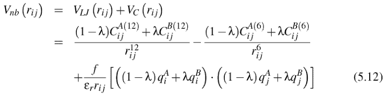
Anmerkungen No source is given.

[73.] Ry/Fragment 071 01

Verschleierung

Untersuchte Arbeit: Seite: 71, Zeilen: 1 ff.

Quelle: Anézo 2003 Seite(n): 157, 158, 159, Zeilen: 157:10ff; 158:1-4,21ff; 159:1-3

III.1.4 Non-equilibrium MD simulations To construct the free energy profile along the membrane normal (z-direction) corresponding to the transfer of the solute from the water layer into the membrane hydrocarbon core, a series of biased simulations is carried out, where an average force method is used to maintain the solute molecules at different positions in the DPPC membrane. This method allows computation of the local diffusion coefficient at the same time, so that permeability coefficients of the solutes in the membrane should be obtained. In order to follow the complete permeation pathway across the membrane, initial configurations are generated by introducing the solute molecules at different depths into the membrane, applying the growing procedure described above. 67 positions along the bilayer normal 1Å apart, are investigated from z0 = – 3.3 to z0=3.3 nm. The solute center of mass is restrained in the z-direction. To limit computational cost, four solute molecules (two per leaflet) are incorporated into the membrane in each starting structure, which reduces the number of simulations from 67 to 17. Simulation conditions are the same as those for the equilibrium MD simulations and a tolerance of constraint 1 x 10-10 nm is used. This leads to using of double precision for calculating of atom coordinates, which rapidly slows down the simulations. Again all bond lengths are kept constant. Each window is equilibrated for 2.5 ns, after which a production trajectory of 12.5 ns is generated. III.2. Results III.2.1 Equilibrium MD simulations Figure 3.3 shows the distribution of the twelve solute molecules in the DPPC membrane at the start and after 35 ns MD simulation for each type of solute. In the final ensemble dimathylarsinic acid molecules are not found in the hydrophobic membrane core anymore and are essentially located in the water layers and at the water/membrane interfaces. The trimethylbismuthane molecules leave the aqueous phase and the membrane interior to adsorb at the water/membrane interface.

[page 157] 5.4.4 Umbrella sampling MD simulations To construct the free energy profile along the membrane normal (z-direction) corresponding to the transfer of the solute from the water layer into the membrane hydrocarbon core, a series of biased simulations is carried out, where an umbrella potential is added to the system to maintain the solute molecules at different positions in the DPPC membrane. In order to follow the complete permeation pathway across the membrane, initial configurations for the umbrella sampling windows are generated by introducing the solute molecules at different depths into the membrane, applying the growing procedure described in the previous section. 67 positions along the bilayer normal, 1 Å apart, are investigated from z0 = —3.3 to z0 = 3.3 nm (the position of the solute COM is defined relative to the position of the DPPC bilayer COM, taken as reference). The solute COM is restrained in the z-direction by a harmonic umbrella potential with a force constant k of 3000 kJ/mol.nm2 (see Equation 5.5), which allows sufficient overlap between adjacent windows. To limit the computational cost, four solute molecules (two per leaflet) are incorporated into the membrane in each starting structure, which reduces the number of simulations from 67 to 17. Simulation conditions are identic to those for the equilibrium MD simulations, with the exception of the type of pressure coupling. [...] Each window is equilibrated for 2.5 ns, after which a production trajectory of 12.5 ns is generated for the umbrella sampling calculations. [...] [page 158] 5.4.5 Constrained MD simulations Constrained simulations allow for the computation of free energy profiles and local diffusion coefficients at the same time, so that permeability coefficients of the solutes in the membrane should be obtained. [...] 5.5.1 Equilibrium MD simulations 5.5.1.1 Time course of solute position Figure 5.9 shows the distribution of the twelve solute molecules in the DPPC membrane at the start (uniform distribution) and after 30 ns MD simulation for each type of solute. In the final ensemble, the polar methylglucose and mannitol molecules are not found in the hydrophobic membrane core anymore and are essentially located in the water layers and at the water/membrane interfaces. At first sight, however, mannitol seems to penetrate somewhat deeper into the membrane than methylglucose does. The salicylic acid molecules leave the aqueous phase and the membrane interior to adsorb, owing to their amphiphilic [page 159] character, at the water/membrane interface, with the polar carboxyl and hydroxyl groups of the molecule interacting with the DPPC headgroups and the hydrophobic benzene ring protruding into the bilayer core.

Anmerkungen No source is given.

[74.] Ry/Fragment 072 01

Verschleierung

Untersuchte Arbeit: Seite: 72, Zeilen: 1-9

Quelle: Anézo 2003 Seite(n): 159, Zeilen: 4 ff.

In order to follow the trajectory of the solute molecules over the simulation from their initial position, the perpendicular motions of the solute center of masses (z-coordinate) have been monitored as a function of time and are depicted in Figures 3.4 and 3.5. On the Figures “hydrocarbon part”, “interface” and “water layer” refer to the initial environment of the molecules. The four molecules dimethylarsinic acid initially located in the hydrocarbon part of the membrane essentially sample the interface. The dimethylarsinic acid molecules initially located in the water layer or at the interface are principally found in the water phase during the simulation. Some of them, however, occasionally migrate to the interfacial region.

In order to follow the trajectory of the solute molecules over the course of the simulation from their initial position, the perpendicular motions of the solute COM (z-coordinate) have been monitored as a function of time and are depicted in Figures 5.10, 5.11, and 5.12. The four methylglucose molecules initially located in the hydrocarbon part of the membrane essentially sample the interfacial region (region 2 and limit between regions 2 and 3). One of the four molecules reaches the water phase after about 15 ns MD. The methylglucose molecules initially located in the water layer or at the interface are principally found in the water phase (region 1) during the simulation. Some of them, however, occasionally migrate to the interfacial region (region 2).

Anmerkungen No source is given

[75.] Ry/Fragment 073 00

Verschleierung

Untersuchte Arbeit: Seite: 73, Zeilen: (entire page)	Quelle: Anézo 2003 Seite(n): 160, Zeilen: -
Figure 3.3. Solute distribution in the DPPC membrane at the start (left) and after 35 ns (right) MD simulation for (a): dimethylarsinic acid and (b): trimethylbismuthane	Figure 5.9: Solute distribution in the DPPC membrane at the start (left) and after 30 ns MD simulation (right) for (a): methylglucose (space fill, orange), (b): mannitol (space fill, magenta), and (c): salicylic acid (space fill, violet).

Anmerkungen No source is given. Only (a) and (c) are used, although they are said to represent different molecules and a longer period of permeation.

[76.] Ry/Fragment 076 01

Verschleierung

Untersuchte Arbeit: Seite: 76, Zeilen: 1 ff.

Quelle: Anézo 2003 Seite(n): 165, Zeilen: 2-11, 21ff

The density distribution profiles along the bilayer normal of the both solute types at the start and during the simulation can be compared in Figure 3.6. The DPPC and water density profiles are also plotted as reference. From these profiles, it can be observed that the density distribution of dimethylarsinic acid exhibits two maxima – one located in the water phase and the other one at the interface. The density distribution of trimethylbismuthane exhibits only one maximum at the DPPC/water interface. Due to its hydrophobicity, the penetration of trimethylbismuthane into the hydrocarbon region of the bilayer is deeper than that of the water. Both density distribution profiles are plotted again in Figure 3.7 for a better comparison. Qualitatively, the probability to find dimethylarsinic acid in the water layer is greater that that to find trimethylbismuthane. The obtained distribution profiles are not completely symmetric with respect to the bilayer center, despite the relative long simulation time of 35 ns. Investigation of solute distribution in the membrane requires intensive statistical sampling, which involves simulation times beyond the reach of equilibrium MD.

5.5.1.2 Solute distribution The density distribution profiles along the bilayer normal of the three solute types at the start and during the simulation can be compared in Figure 5.14. The DPPC and water density profiles are also plotted as reference. From these profiles, it can be observed that the density distribution of methylglucose and mannitol exhibits two maxima: one is located in the water phase (region 1), the other one at the interface, at the limit between regions 2 and 3. The density distribution of salicylic acid exhibits only one maximum, also located at the limit between regions 2 and 3. Methylglucose and mannitol penetrate into the membrane as long as water is present. Due to its partial hydrophobicity, the penetration of salicylic acid into the hydrocarbon region of the bilayer is somewhat deeper than that of water. The solute density distribution profiles are plotted again in Figure 5.15 and compared to those of the choline, phosphate, and carboxyl moieties of the DPPC headgroups. [...] Figure 5.17 is a close-up shot of the solute density distribution profiles which allows for a better comparison of the three profiles. Qualitatively, the probability to find methylglucose in the water layer is greater than that to find mannitol and mannitol seems to interact stronger than methylglucose with the DPPC headgroups in the interfacial region. It can be also noticed from Figure 5.17 that the obtained distribution profiles are not completely sym­metric with respect to the bilayer center, despite the relative long simulation time (30 ns). A thorough investigation of solute distribution in the membrane requires intensive statistical sampling, which involves simulation times beyond the reach of equilibrium MD.

Anmerkungen No source is given.

[77.] Ry/Fragment 079 08

Verschleierung

Untersuchte Arbeit: Seite: 79, Zeilen: 8-11

Quelle: Anézo 2003 Seite(n): 171, Zeilen: 5-10

From the density distribution profiles obtained from the equilibrium MD, simulations, free energy profiles can be calculated, at least in the water and in the interfacial regions, using the relation ΔG(z)= – RcTlnρ(z), where ρ(z), represents the density distribution of the solute in the water/DPPC system. These profiles are compared to those obtained from [the non-equilibrium MD simulations in Figure 3.9 and 3.10. Good agreement is found between both methods.]

[page 171] From the density distribution profiles obtained from the equilibrium MD simulations, free energy profiles can be calculated, at least in the water and interfacial regions, using the relation ΔG(z) = — RcT ln ρ (z), where ρ (z) represents the density distribution of the solute in the water/DPPC system. These profiles are compared to those obtained from the umbrella sampling simulations in Figure 5.19. A good agreement is generally found between both methods.

Anmerkungen No source is given.

[78.] Ry/Fragment 080 01

Verschleierung

Untersuchte Arbeit: Seite: 80, Zeilen: 1-5 (entire page except figure)

Quelle: Anézo 2003 Seite(n): 171, Zeilen: 171:8-9, 11-15

[These profiles are compared to those obtained from] the non-equilibrium MD simulations in Figure 3.9 and 3.10. Good agreement is found between both methods. Validation of the calculated free energy barriers is not possible, since no experimental data about solute partitioning at water/membrane interfaces is available from the literature.

These profiles are compared to those obtained from the umbrella sampling simulations in Figure 5.19. A good agreement is generally found between both methods. [...] Validation of the calculated free energy barriers is difficult, since few experimental data about solute partitioning at water/membrane interfaces are available from the literature. Recently, water/dodecane partition coefficients have been determined by Bas et al. [218], using the shake flask method, for a series of drug and drug-like molecules, including α-D-glucose. [218] D. Bas, D. Dorison-Duval, S. Moreau, P. Bruneau, and C. Chipot. J. Med. Chem., 45:151–159, 2002.

Anmerkungen No source is given. Similar but not identical figures follow this text (Ry: 3.9, Anézo: 5.19).

[79.] Ry/Fragment 083 01

Verschleierung

Untersuchte Arbeit: Seite: 83, Zeilen: 1 ff. (entire page)

Quelle: Anézo 2003 Seite(n): 48, 49, Zeilen: 48: 9-17,26-31; 49: 1-7,15-21

III.3. Discussion The absorption of compounds by passive diffusion can be reasonably well predicted on the basis of their chemical properties. The presence of polar and charged functional groups a substantial number of hydrogen-bonding sites, high molecular weight, and large polar surface area are generally associated with poor membrane permeability. In many cases, however, the consideration of permeant properties alone proves to be not sufficient for a proper evaluation of permeation data: permeability coefficients may be overestimated or, on the contrary, underestimated. Another important factor to take into account is, indeed, the nature and the permeability of the membranes that have to be crossed. Independently on the type of membranes, membrane fluidity is generally correlated with membrane permeability and the degree of fluidity influences largely the ability of a solute to pass through the membrane. All factors increasing membrane fluidity may also enhance membrane permeability. The formation of structural discontinuities in the bilayer, even only transiently, increases membrane permeability, especially in the case of small permeants, which can jump from one discontinuity to another. Such discontinuities are for instance observed in the presence of unsaturated lipid chains, which generate packing defects in the bilayer interior. Phase separation phenomena within the membrane can also increase permeation processes. Under certain conditions, indeed, the bilayer organization can be interrupted by non-bilayer phases as well as by bilayer phases of different compositions. The regions of mismatch between these coexisting phases can be viewed as fractures within the membrane. Such topological discontinuities may promote solute permeation through the membrane. During the diffusion process, the molecules may exhibit a well-defined orientation with respect to the bilayer normal and adopt specific conformations, different from those generally found in an aqueous medium. This can be related to the highly structured environment of the bilayer and to its difference in polarity compared with water. Because of the anisotropic properties of membranes, their complex structural organization and chemical composition, and their asymmetry, the transport cannot be correctly described [by single parameters.]

[page 48] The absorption of compounds by passive diffusion can be reasonably well predicted on the basis of their physicochemical properties. The presence of polar and charged functional groups, low octanol/water partitioning, a substantial number of hydrogen-bonding sites, high molecular weight, and large polar surface area are generally associated with poor membrane permeability. In many cases, however, the consideration of drug properties alone proves to be not sufficient for a proper evaluation of permeation data: permeability coefficients may be overestimated or, on the contrary, underestimated. Another important factor to take into account is, indeed, the nature and the permeability of the membranes that have to be crossed by the drug. [...] Independently on the type of membranes, membrane fluidity is generally correlated with membrane permeability and the degree of fluidity influences largely the ability of a solute to pass through the membrane. All factors increasing membrane fluidity (see Section 1.2.4.3, page 39) may also enhance membrane permeability. The formation of structural discontinuities in the bilayer, even only transiently, increases membrane permeability, especially in the case of small permeants which can jump from one discontinuity to another. Such disconti- [page 49] nuities are for instance observed in the presence of unsaturated lipid chains which generate packing defects in the bilayer interior. Phase separation phenomena within the membrane can also increase permeation processes. Under certain conditions, indeed, the bilayer organization can be interrupted by non-bilayer phases as well as by bilayer phases of different compositions. The regions of mismatch between these coexisting phases can be viewed as fractures within the membrane. Such topological discontinuities may promote solute permeation through the membrane. [...] During the diffusion process, drug molecules may exhibit a well-defined orientation with respect to the bilayer normal and adopt specific conformations, different from those generally found in an aqueous medium. This can be related to the highly structured environment of the bilayer and to its difference in polarity compared with water. Because of the anisotropic properties of membranes, their complex structural organization and chemical composition, and their asymmetry, drug transport cannot be correctly described by single parameters such as octanol/water partition coefficients.

Anmerkungen The source is not given

[80.] Ry/Fragment 084 01

Verschleierung

Untersuchte Arbeit: Seite: 84, Zeilen: 1 ff.

Quelle: Anézo 2003 Seite(n): 49, 182, 183, Zeilen: 49:18-26; 182:2-10; 183:12-24

[Because of the anisotropic properties of membranes, their complex structural organization and chemical composition, and their asymmetry, the transport cannot be correctly described] by single parameters. A detailed knowledge of membrane characteristics is fundamental for a proper estimation of permeation rates. This is especially true for amphiphilic molecules, having a hydrophobic and a hydrophilic gravity center: their orientation within the membrane may be strongly affected by the structural organization of the bilayer as well as by the possible electrostatic and van der Waals interactions with the membrane components. The simulations performed show that the permeation process of organometallic compounds through a phospholipid membrane is essentially determined by the free energy barrier that results from the breakage of H-bonds between the solutes and water and between the solutes and the polar lipid headgroups and from the loss of electrostatic interactions. In the DPPC membrane, the carbonyl groups of the glycerol-ester linkages seem to play an important role in the permeation process: they have the polar and hydrogen-bonding function closest to the bilayer center and attract water as well as polar solutes close to the hydrophobic hydrocarbon region of the bilayer. They also play a determinant role in the adsorption, as is shown in the simulations with trimethylbismuthane. The full description of permeation processes requires not only the knowledge of the underlying free energy behavior, but also of the local diffusion coefficient, both quantities contributing to the global permeation rate. With the simulations based on the average force method on constrained particle is possible to estimate free energy profile, local diffusion coefficient and permeation coefficient, however, corresponding force curves are very noisy and further work with them is particularly difficult. The reasons could be several. The theoretical derivation of the permeability coefficient described in Section II.4.2, rests on the assumption that the thermodynamic gradient can be considered constant over the correlation distance of the particle. In the strict sense, this method is only valid for permeants of relative small size and for energy barriers, which do not exhibit too steep slopes. The molecules, on which the method was experimented, are probably too big for this method, and their permeation cannot be treated as an equilibrium process. A permeant of the size of the molecules studied does not get to the top of the energy barrier [slowly and in constant equilibrium, but is driven over it quickly by its momentum, inertia effects becoming important in the case of a large permeant.]

[page 49] Because of the anisotropic properties of membranes, their complex structural organization and chemical composition, and their asymmetry, drug transport cannot be correctly described by single parameters such as octanol/water partition coefficients. A detailed knowledge of membrane characteristics is fundamental for a proper estimation of permeation rates. This is especially true for amphiphilic drugs, having a hydrophobic and a hydrophilic gravity center: their orientation within the membrane may be strongly affected by the structural organization of the bilayer as well as by the possible electrostatic and van der Waals interactions with the membrane components. [page 182] 5.6 Discussion The simulations performed show that the permeation process of polar solutes through a phospholipid membrane is essentially determined by the free energy barrier that results from the breakage of H-bonds between the solutes and water and between the solutes and the polar lipid headgroups and from the loss of electrostatic interactions. In the DPPC membrane, the carbonyl groups of the glycerol-ester linkages seem to play an important role in the permeation process: they have the polar and hydrogen-bonding function closest to the bilayer center and attract water as well as polar solutes close to the hydrophobic hydrocarbon region of the bilayer. They also play a determinant role in the adsorption of amphiphilic solutes, as shown in the simulations with salicylic acid. [page 183] The full description of permeation processes requires not only the knowledge of the underlying free energy behavior, but also of the local diffusion coefficient, both quantities contributing to the global permeation rate. Unfortunately, the simulations based on the average force method on constrained particle, aimed at calculating permeability coefficients, were not successful. The theoretical derivation of the permeability coefficient described in Section 5.2.2.2, page 144, rests on the assumption that the thermodynamic gradient can be considered constant over the correlation distance of the particle. In the strict sense, this method is only valid for permeants of relative small size and for energy barriers which do not exhibit too steep slopes [135, 194]. The molecules, on which the method was experimented, are probably too big for this method, and their permeation cannot be treated as an equilibrium process. A permeant of the size of the molecules studied does not get to the top of the energy barrier slowly and in constant equilibrium, but is driven over it quickly by its momentum, inertia effects becoming important in the case of a large permeant. [135] S. J. Marrink and H. J. C. Berendsen. J. Phys. Chem., 98:4155–4168, 1994. [194] S. J. Marrink and H. J. C. Berendsen. J. Phys. Chem., 100:16729–16738, 1996.

Anmerkungen The source is not given.

[81.] Ry/Fragment 085 01

Verschleierung

Untersuchte Arbeit: Seite: 85, Zeilen: 1-6

Quelle: Anézo 2003 Seite(n): 182, 183, Zeilen: 182: 30 ff. - 183: 1, 22-24

[A permeant of the size of the molecules studied does not get to the top of the energy barrier] slowly and in constant equilibrium, but is driven over it quickly by its momentum, inertia effects becoming important in the case of a large permeant. The discrepancies can also probably be attributed to parameters adopted for DPPC molecule, issued from extensible systematic force field, which may be not optimal in context of free energy calculations to properly describe the interactions between hydrocarbon chains of DPPC molecule and organometallic compounds.

[page 182] The discrepancy can probably be attributed to the parameters adopted for salicylic acid, issued from the standard OPLS force field, which may be not optimal in the context of free energy calculations to properly describe the interactions between the aromatic ring of the acid and [page 183] the hydrocarbon chains of DPPC. [...] [...] A permeant of the size of the molecules studied does not get to the top of the energy barrier slowly and in constant equilibrium, but is driven over it quickly by its momentum, inertia effects becoming important in the case of a large permeant.

Anmerkungen No source is given.

[82.] Ry/Fragment 087 01

Verschleierung

Untersuchte Arbeit: Seite: 87, Zeilen: 1ff (entire page)

Quelle: Anézo 2003 Seite(n): 183, 184, Zeilen: 183: last paragraph; 184: 1ff

IV. General conclusions Molecular dynamics simulations can test theoretical notions and complement experimental techniques to further the conceptual understanding of the solute distribution and dynamics in lipid membranes. The free energy computations described in the thesis offer more than a simple estimation of the height of the energy barrier associated to the permeation process. By constructing the complete free energy profile across the membrane, details of the solute-membrane interactions are brought in light and help to rationalize the mechanisms of transport. The average force method, which describes the full permeation process, including both the partitioning and diffusion contributions, proved to be very informative, helping to better understand the permeation processes. The computational effort that warrants accurate, converged free energies is, however, prohibitive and remains, in large measure, incompatible with the investigation of large sets of compounds.

5.7 Conclusion Hence, MD simulations can test theoretical notions and complement experimental techniques to further the conceptual understanding of the solute distribution and dynamics in lipid membranes. The free energy computations described in this chapter offer more than a [page 184] simple estimation of the height of the energy barrier associated to the permeation process. By constructing the complete free energy profile across the membrane, details of the solute-membrane interactions are brought in light and help to rationalize the mechanisms of transport. The computational effort that warrants accurate, converged free energies is, however, prohibitive and remains, in large measure, incompatible with the investigation of large sets of compounds. In the present study, a compromise had to be found between the computational cost and the need for adequate sampling. The constrained method tested for the description of the full permeation process, including both the partitioning and diffusion contributions, was not successful. Nonetheless, the realization of the limits of the method, i.e. the difficulty to extract a permeability coefficient from the data, proved to be very informative, helping to better understand the permeation process.

Anmerkungen The source is not mentioned.

[83.] Ry/Fragment 088 01

Verschleierung

Untersuchte Arbeit: Seite: 88, Zeilen: 1 ff.

Quelle: Anézo 2003 Seite(n): 185, 186, Zeilen: 185:1-12,20-22; 186: 1-8

V. Summary The aim of this thesis was to investigate the permeation of small organometallic molecules through a membrane computer model at a molecular level by means of molecular dynamics simulations. As a first step, a realistic model for a typical biological membrane was developed. As phospholipid bilayers provide simple but very informative model systems, a pure phospholipid bilayer system, containing a single type of phospholipid (dipalmitoylphosphatidylcholine or DPPC), was simulated in the biologically relevant liquid crystalline state. The simulated DPPC membrane patch consists of 200 lipids (100 per leaflet) and about 5800 water molecules. Emphasis was laid on properties that are thought to play an important role in permeation processes, such as membrane density, ordering degree of the lipid acyl chains, or lipid mobility. As a second step, the permeation processes of a dimethylarsinic acid and trimethylbismuthane through the DPPC membrane model were studied. These compounds were chosen because they are one of the simplest widely distributed in nature organometallic compounds, containing arsenium and bismuth. As permeation processes are too slow on the time scale accessible to the molecular dynamic technique, they cannot be directly followed. Equilibrium molecular dynamic simulations were first carried out to gain insight into the solute partitioning behavior within the membrane. Non-equilibrium simulations, based on the average force method, were then undertaken to quantify the free energy barrier to be overcome by the permeants for their translocation from the water phase into the membrane interior.

[page 185] Summary The aim of this thesis was to investigate the permeation of small drug-like molecules through a membrane computer model at a molecular level by means of molecular dynamics (MD) simulations. As a first step, a realistic model for a typical biological membrane was developed. As phospholipid bilayers provide simple but very informative model systems, a pure phospholipid bilayer system, containing a single type of phospholipid (dipalmitoylphosphatidylcholine or DPPC), was simulated in the biologically relevant liquid crystalline state. DPPC was chosen in reason of its prevalence in mammalian plasma membranes and of the large amount of experimental data available on phosphatidylcholine membranes. The simulated DPPC membrane patch consists of 128 lipids (64 per leaflet) and about 4000 water molecules. [...] Emphasis was laid on properties that are thought to play an important role in permeation processes, such as membrane density, ordering degree of the lipid acyl chains, or lipid mobility. [...] [page 186] As a second step, the permeation process of a sugar (methylglucose), a polyalcohol (mannitol), and a drug-like molecule (salicylic acid) through the DPPC membrane model was studied. As permeation processes are too slow on the time scale accessible to the MD technique, they cannot be directly followed. Equilibrium MD simulations were first carried out to gain insight into the solute partitioning behavior within the membrane. Non-equilibrium simulations, based on the umbrella sampling approach, were then undertaken to quantify the free energy barrier to be overcome by the permeants for their translocation from the water phase into the membrane interior.

Anmerkungen

Quellen

[1.] Quelle:Ry/Anézo 2003

Autor	Céline Anézo
Titel	Molecular models for drug permeation across phospholipid membranes
Ort	Düsseldorf
Jahr	2003
Anmerkung	Düsseldorf, Univ., Diss., 2003
URL	http://d-nb.info/969487479/34
Literaturverz.	ja
Fußnoten	ja

[2.] Quelle:Ry/Biosym MSI - Integration Algo 1995

Titel	Molecular Dynamics - Integration Algorithms
Jahr	1995
Anmerkung	Chapter from "The Discover Program - Documentation" Release 95.0/3.00, October 1995
URL	http://www.uoxray.uoregon.edu/local/manuals/biosym/discovery/General/Dynamics/Integration_Algo.html
Literaturverz.	nein
Fußnoten	nein

[3.] Quelle:Ry/Accelrys Inc. - Forcefield-Based Simulations 1998

Autor	Accelrys Inc.
Titel	Forcefield-Based Simulations
Ort	San Diego
Datum	September 1998
Anmerkung	http://www.esi.umontreal.ca/accelrys/life/insight2000.1/getdown.html
URL	http://www.esi.umontreal.ca/accelrys/pdf/ffbs980.pdf